FILTER Function in Microsoft Excel – The Easy Way

The FILTER function is a flexible tool that allows users to extract specific data from a larger dataset based on specific criteria. It saves users time and effort by allowing them to quickly retrieve specific information instead of manually searching through large amounts of rows. It offers a simple and efficient method to extract the desired data effortlessly.

The FILTER function syntax:

The data range – the entire dataset to be filtered

The include range – the column or columns that contain the criteria for filtering

The criteria range – the specific values to search for

In this article, we will explore these methods on how to use Excel’s FILTER function with ease:

Let’s look at these methods thoroughly!

Download the Excel Workbook below to follow along and understand How to Use Substrings in Microsoft Excel –

download excel workbookFILTER-FUNCTION.xlsx

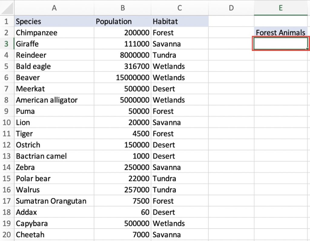
Imagine you are a biologist in charge of a dataset about various animal species in a specific region. On hand, you have data on different animals, including their species, population count, and habitat type. Let’s create an example using the basic FILTER function:

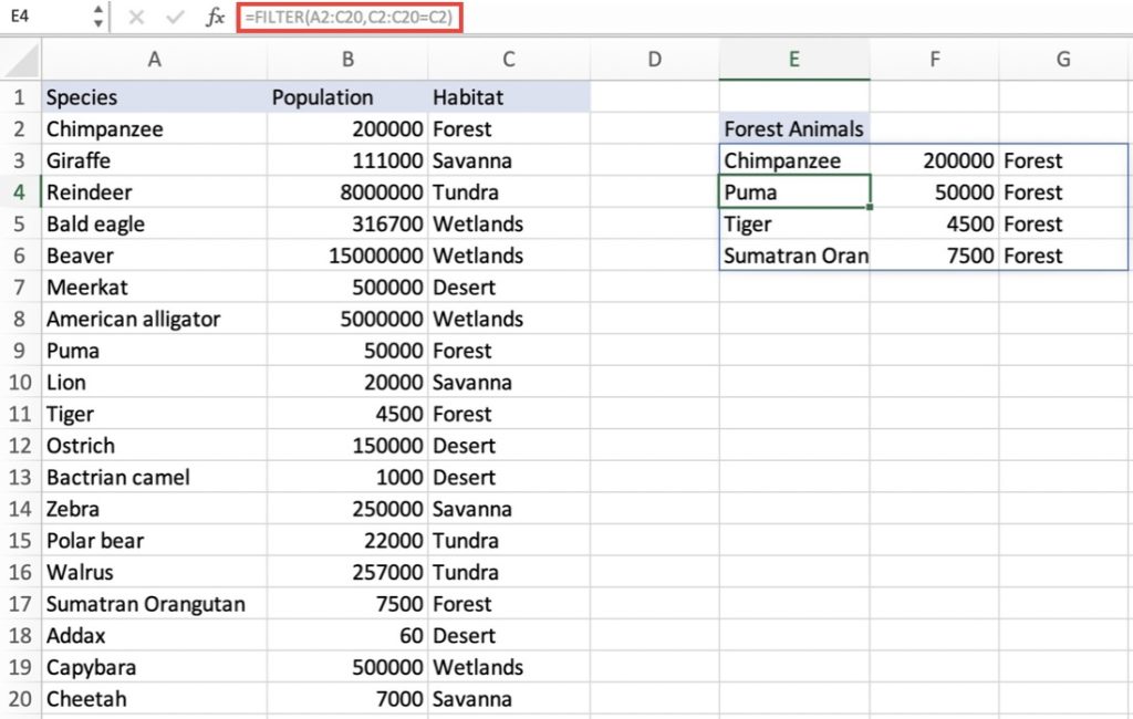
Let’s say you want to filter the data to focus on a specific habitat type, such as Forest.

Select an empty cell where you want the filtered data to appear.

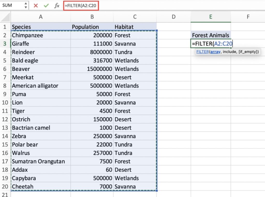
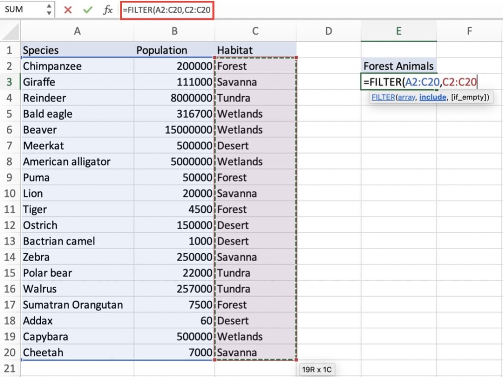
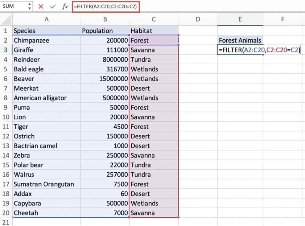
In the formula bar, enter =FILTER(data_range, include_range = criteria_range).

Replace “data_range” with the range of your entire dataset, which includes the three columns of animal data.

For “include_range,” select the range corresponding to the habitat type column.

Lastly, for “criteria_range,” specify the habitat type you want to filter by. In our case, it is Forest.

Press Enter.

The filtered data, containing only the animals that inhabit forests, will populate the selected cell.

This way, you can focus on analyzing the population counts and study the diversity of the animals that live in the forest without being distracted by data related to other habitats.

FILTER with Multiple Criteria

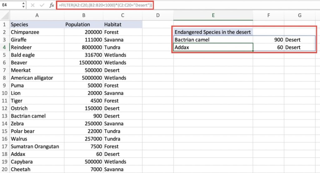
Now, suppose you want to filter the data further to identify the endangered species within the desert habitat. To achieve this, you can use an additional criterion.

In the formula bar, enter the following formula:
=FILTER(A2:C20,B2:B20 <1000)*(C2:C20=”Desert”))

This formula filters the dataset based on two conditions: population count less than 1000 (B2:B20 < 1000) and habitat type equal to “Desert” (C2:C20 = “Desert”). The * symbol acts as the logical AND operator, ensuring that both conditions are met for a row to be included in the filtered result.

As you can see, the data will now display only the animals that inhabit forests and have a population count below 1,000, indicating endangered species.

Excel FILTER Multiple Conditions with OR

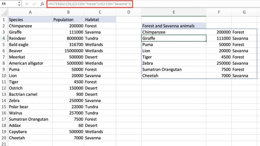
Let’s say you want to filter the data for animals in either the “Forest” or “Savanna” habitat types.

Select an empty cell where you want the filtered data to appear.

In the formula bar, enter the following formula:
=FILTER(A2:C20, (C2:C20 = “Forest”) + (C2:C20 = “Savanna”))

Press Enter.

Now you can acquire data containing animals from either the Forest or Savanna habitats.

FILTER function with IF

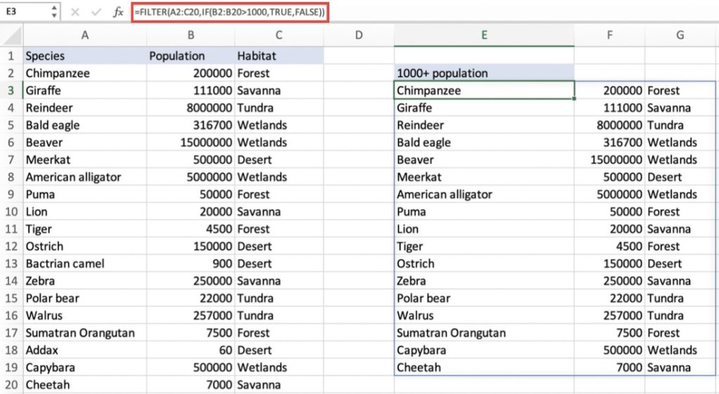
What if you want to filter the data to display only the animals with a population count greater than 1,000? This is where the IF formula comes in handy in tandem with the FILTER function.

Select an empty cell where you want the filtered results to appear.

Enter =FILTER(A2:C20, IF(B2:B20>1000, TRUE, FALSE))

This formula combines the FILTER function and the IF function. It filters the range A2:C20 based on the condition specified in the IF function.

Press Enter.

The FILTER function uses the specified data range (A2:C20) as the dataset to filter. The IF function is used as the include range, where it checks the population counts in column B and returns TRUE if the count is greater than 1,000, and FALSE if it is not.

As a result, the FILTER function displays only the rows of animals that meet the specified criteria of having a population count greater than 1,000.

FILTER function with UNIQUE

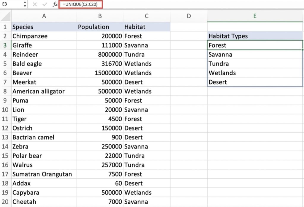
Let’s say you want to extract the unique habitat types from the dataset.

Select an empty column where you want the unique habitat types to appear.

In the formula bar, enter:

=UNIQUE(C2:C20) in the first cell of that column.

Press Enter.

By following these steps, you can easily extract the unique habitat types from your animal data. This helps you identify the distinct habitat types present in your dataset without any repetitions.

FILTER function with SORT

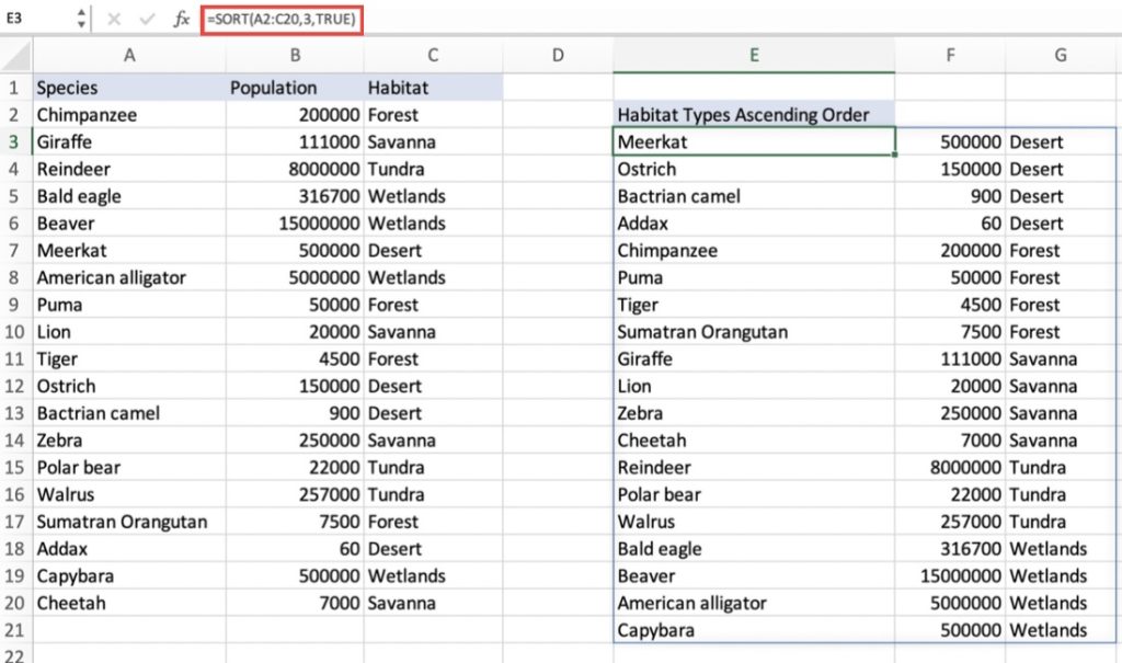
Let’s say you want to sort the data based on the habitat types in ascending order.

Select an empty range where you want the sorted data to appear (including all columns).

Enter the following formula in the first cell of the selected range:

=SORT(A2:C20, 3, TRUE)


This formula sorts the dataset based on the habitat type column in ascending order.

Press Enter.

Now you can organize the data and view animals grouped by their respective habitat types.

There you have it! By taking advantage of the FILTER function, you can easily analyze data without having to sift through irrelevant information.