The Ultimate Guide to Filter Function with Multiple Criteria in Excel

When working with large datasets in Excel, one of the biggest challenges is narrowing down the data to exactly what you need. That’s where the FILTER function comes into play. It allows us to pull specific data that meets certain criteria, making it a powerful tool for sorting through complex datasets. But what happens when we have multiple criteria to filter by?

Luckily, Excel’s FILTER function can handle that, too. In this guide, I’ll walk you through how to use the FILTER function with multiple criteria, and by the end, you’ll be a pro at extracting data precisely the way you want it.

Key Takeaways:

• The FILTER function in Excel extracts data based on specified criteria, making it ideal for narrowing down large datasets.
• You can combine multiple criteria using logical operators like AND and OR for more complex filtering.
• Excel tables enhance the FILTER function by dynamically updating with new data and improving overall functionality.
• Nesting FILTER functions allow you to filter non-adjacent columns, providing flexibility in data extraction.
• Backup strategies are crucial before applying filters to avoid potential data loss during analysis.

 

Unlocking the Power of Excel Filter Function

What Is the FILTER Function?

At its core, the FILTER function in Excel extracts data based on a given condition. For example, if I wanted to filter out a list of sales to only show those above a certain value, I could use the FILTER function to do that quickly.

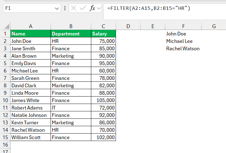
The syntax is: =FILTER(array, include, [if_empty])

• Array: The range of data you want to filter.
• Include: The condition(s) or criteria to apply.
• [if_empty]: Optional. What to return if no values meet the criteria (e.g., “No Data”).

 

Why Use Multiple Criteria?

In the real world, we rarely work with simple datasets that have only one criterion. For example, when working on a customer analysis report, I might need to pull data for sales that happened during a specific time period and for specific product categories.

That’s where using multiple criteria becomes essential. Fortunately, Excel gives us the flexibility to combine multiple conditions using logical operators.

Logical Operators for Multiple Criteria

When I’m dealing with multiple conditions, I can use logical operators such as AND and OR to specify exactly how I want the criteria to work.

• AND logic: All conditions must be met. For example, if I want to filter for sales greater than $500 and occurring in 2023.
• OR logic: At least one of the conditions must be met. For example, sales greater than $500 or occurring in 2023.

Now, let’s jump into some practical examples to see how this works in Excel.

 

Example of Filter Function with Multiple Criteria

Crafting Filters with Multiple AND Criteria

When we craft filters with multiple AND criteria in Excel, we’re setting strict parameters. To visualize, each criterion forms a gate, and a row of data must pass through every gate to make it into our final filtered list. It’s a sequence of ‘checks’ in which all conditions must be true.

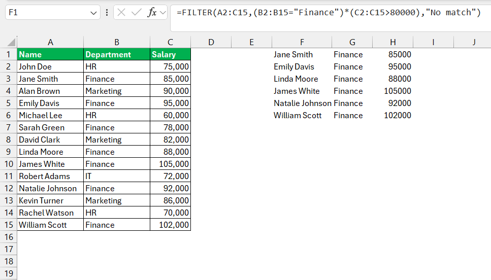
For instance, in the formula =FILTER(A2:C15,(B2:B15="Finance")*(C2:DC15>80000),"No match"), we’re searching for employees in the Finance department with salaries above $80,000.

Each condition adds a layer of specificity, ensuring that the data we work with is exactly what we need for our analysis.

Manipulating Data with Multiple OR Criteria

Utilizing OR criteria broadens our filtering approach, where rows meet any one of our set conditions to be displayed. Imagine a net with wider meshes, capable of catching a larger variety of fish. By summing Boolean expressions with plus signs, we allow for greater inclusivity in our filtering.

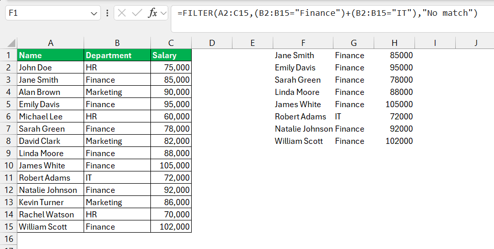
A formula such as =FILTER(A2:C15, (B2:B15="Finance") + (B2:B15="IT"), "No match") would extract records where the department is equal to either HR or Finance.

This flexibility lets us cast a wider net when gathering data points that fall into multiple, varied categories.

 

Real World Examples – Master Filter Function with Multiple Criteria

Case Study: Filtering Sales Data by Date and Value

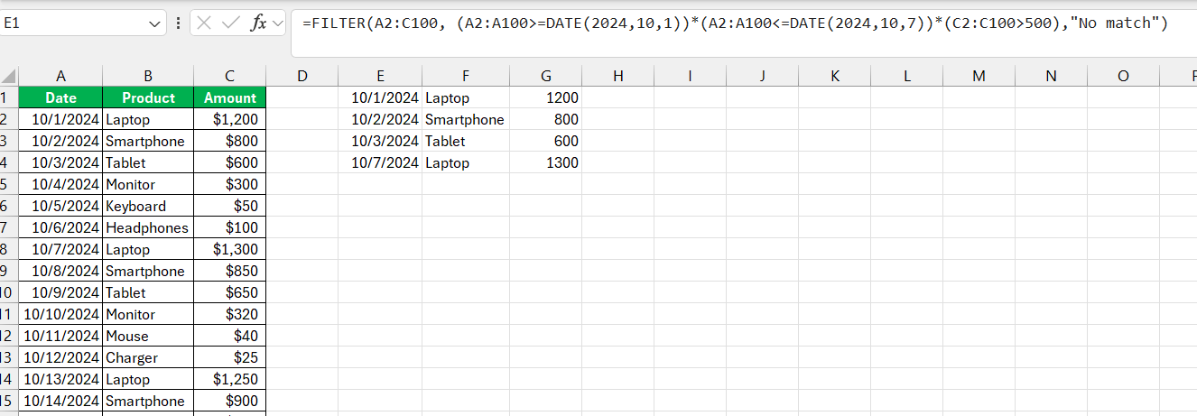
In a case study I examined, a company sought to analyze its sales data by both date and value, and the FILTER function proved instrumental. They used expressions like =FILTER(A2:C100, (A2:A100>=DATE(2024,10,1))*(A2:A100<=DATE(2024,10,7))*(C2:C100>5000),"No match") to isolate transactions from the 1st 7 days of October month with sales over $5000.

The result was a focused data set from which they could derive trends and patterns, informing strategic business decisions. It’s this precise targeting that can elevate a good business strategy to a great one.

Problem-Solving: Using Filter on Non-Adjacent Columns

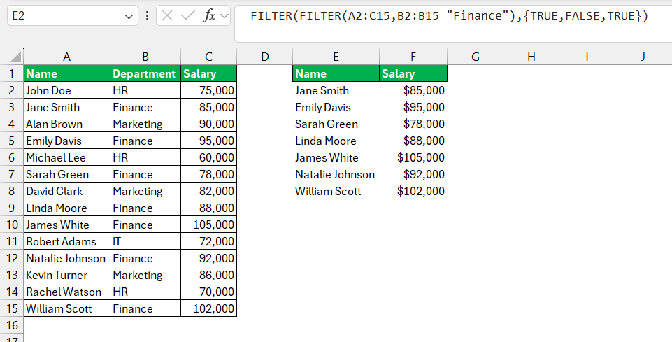
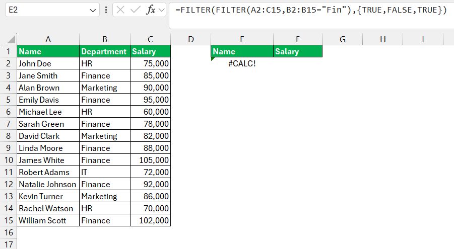
It’s quite the riddle at times—how to use Excel’s FILTER function on non-adjacent columns. The clever trick lies in nesting two FILTER functions together. For example, to display non-contiguous columns, such as Names (first column) and Salary (third column), the formula would look something like this: =FILTER(FILTER(A2:C15,B2:B15="Finance"),{TRUE,FALSE,TRUE}).

The key to unlocking this is the use of an array constant that includes TRUE for columns to keep and FALSE for those to exclude. This workaround ensures I can pull precisely the information I need, deftly sidestepping any adjacent column restrictions.

 

Troubleshooting Common Hurdles

No Data Matches the Criteria

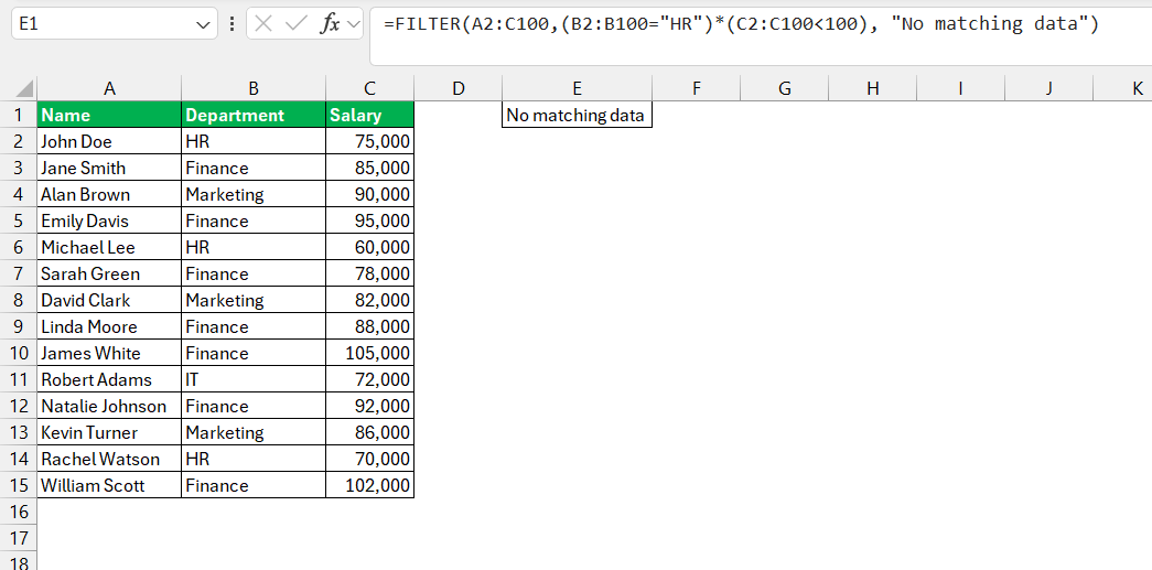
Sometimes, when applying multiple criteria, I end up with no data matching my filters. To handle this, I always use the third argument of the FILTER function ([if_empty]), which displays a custom message if no data meets the conditions.

For example:

=FILTER(A2:C100, (B2:B100=”HR”) * (C2:C100<100), “No matching data”)

#VALUE! Error

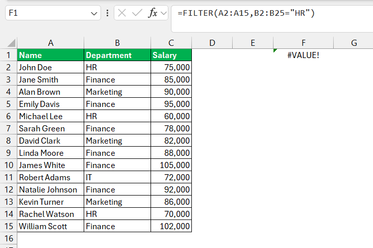
If I see the #VALUE! error, it often means the ranges in the formula don’t match in size. Double-check that all ranges (e.g., A2 and C2) have the same number of rows.

Decoding Errors: #SPILL, #CALC!, and Others

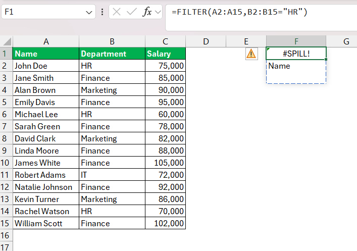
Decoding Excel errors can feel like cracking a secret code, but knowing the common culprits can simplify the process. A frequent disruptor is the #SPILL error, often indicating a blockage—another cell’s content is preventing the filtered data from ‘spilling’ into the expected range. Clearing these cells usually resolves the issue.

As for #CALC!, it points to a calculation problem, perhaps a circular reference or an overload from a massive array.

Reviewing the formula logic for these errors and ensuring no part of the formula conflicts with another can pave the way towards a smooth functioning spreadsheet once more.

 

Tips and Best Practices

Keeping Your Data Dynamic with Excel Tables

Embracing Excel tables is a game-changer for data dynamism. By converting a data range into a table, we ensure that any addition or change in our data automatically extends any related filters. It’s like setting up a smart, self-updating system where the FILTER function adapts in real time, maintaining the accuracy and relevance of our analysis.

Furthermore, Excel tables also come with built-in features like sorting, filtering, and stylish formatting, which enhance both the functionality and the visual appeal of our datasets.

Preventing Data Loss – Backup Strategies Before Applying Filters

Before diving into data manipulation with filters, safeguarding our data is paramount. The cardinal rule I abide by is to always have a robust backup strategy in place. This might mean creating a duplicate of the dataset or employing Excel’s version control features.

In either case, the goal is to preserve the original data, such that if any misstep occurs during the filtering process, we can revert to the unaltered state with ease. Prevention, in this case, far outstrips the need for a cure, providing peace of mind as we delve into intricate data analysis.

 

FAQs

How Can I Use Multiple Criteria in One Column with the Filter Function?

To use multiple criteria within a single column using the FILTER function, we can combine conditions using the “+” symbol for OR logic, or the “*” symbol for AND logic. For example, =FILTER(A2:A10, (B2:B10="Criteria1") + (B2:B10="Criteria2")) returns rows where the value in column B is either “Criteria1” or “Criteria2”. Remember that our criteria should be constructed carefully to ensure they’re returning the correct rows from our dataset.

What Are the Limitations of the Filter Function with Multiple Criteria Complexity?

The FILTER function, while powerful, isn’t without constraints. One primary limitation arises with complexity—it’s built for vector operations, meaning each criterion is processed one row at a time and may not support multi-row complex criteria. Additionally, it can’t directly reference different sheets or workbooks in a single formula. For intricate, multi-layered criteria that surpass basic Boolean logic, we may need to seek other features or functions, such as Power Query for more complex data-shaping tasks.

What is the filter function?

The FILTER function is a dynamic feature in Excel that allows us to extract data based on specific criteria from a given range. It sifts through the data, returning an array that meets our set conditions. What sets it apart is its dynamic nature—as the input data changes, the FILTER function automatically adjusts the output, ensuring up-to-date results without needing to manually reapply the filter. It’s an essential function for managing large datasets and conducting targeted data analysis.

What is the dynamic filter function in Excel?

The dynamic filter function in Excel refers to the FILTER function, an elegant addition to the Excel formula roster that dynamically updates its output. When changes occur in the underlying data or within the criteria specified, the results reshuffle automatically to reflect the latest information. This function is especially powerful in Excel 365, where the calculation engine supports dynamic arrays, making real-time data manipulation and analysis both feasible and efficient.

How do you usually filter in Excel?

Typically, I filter in Excel using the built-in ‘Sort & Filter’ options accessible from the ‘Data’ tab. It’s direct and user-friendly—I select the range or a table I want to filter and then toggle the filter icons in the column headers to set my criteria for text values, numbers, dates, or even colors. However, when it comes to dynamic or complex filtering, where I need the results to update automatically as data changes, I use the FILTER function. It offers a formula-based approach and grants me more nuanced control over the output, adeptly adapting to new data without the need for manual intervention.