Power Query or Get & Transform (In Excel 2016) lets you perform a series of steps to transform your Excel data. One of the steps it allows you to take is to format text with multiple ways.
For our example, let us go over the most common usages of format text:
- Upper case
- Lower case
- Capitalize each word
- Trim
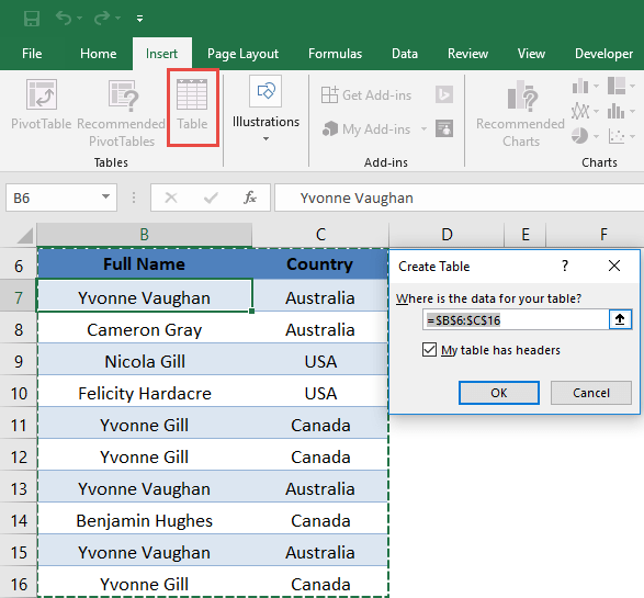
STEP 1: Select your data and turn it into an Excel Table by pressing the shortcut Ctrl + T or by going to Insert > Table
STEP 2: Go to Data > Get & Transform > From Table (Excel 2016) or Power Query > Excel Data > From Table (Excel 2013 & 2010)
Excel 2016:
Excel 2013 & 2010:
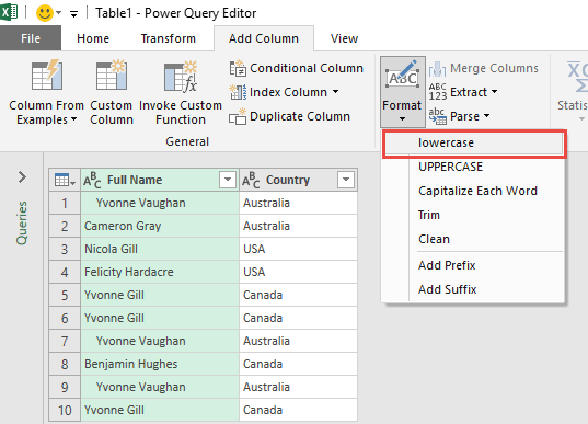
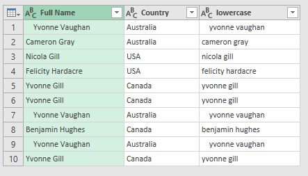
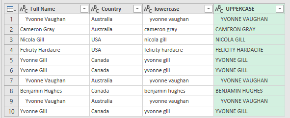
STEP 3: This will open up the Power Query Editor. Let us try to convert to lower case.
Make sure the Full Name column is selected. Go to Add Column > From Text> Format > lowercase
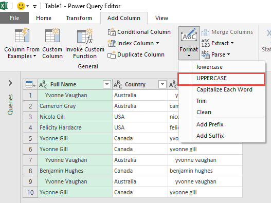
STEP 4: Let us try to convert to upper case.
Make sure the Full Name column is selected. Go to Add Column > From Text> Format > UPPERCASE
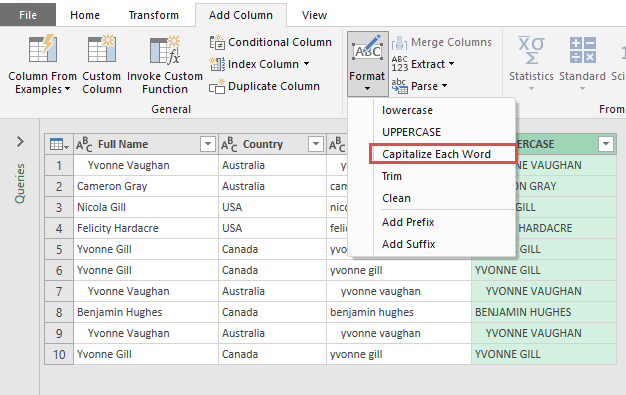
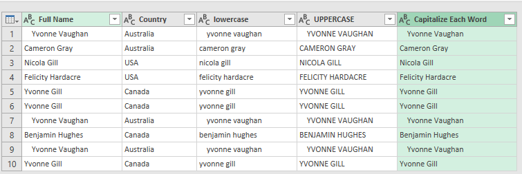
STEP 5: Let us now capitalize each word.
Make sure the UPPERCASE column is selected. Go to Add Column > From Text> Format > Capitalize each word
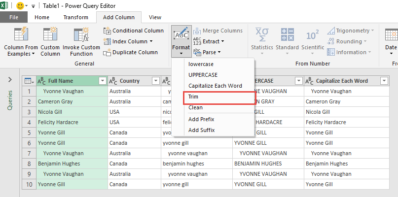
STEP 6: Let us now try out trimming the text to rid of the extra spaces.
Make sure the Full Name column is selected. Go to Add Column > From Text> Format > Trim
We have now formatted our text in Power Query in multiple ways!
How to Format Text in Excel Using Power Query

Bryan
Bryan Hong is an IT Software Developer for more than 10 years and has the following certifications: Microsoft Certified Professional Developer (MCPD): Web Developer, Microsoft Certified Technology Specialist (MCTS): Windows Applications, Microsoft Certified Systems Engineer (MCSE) and Microsoft Certified Systems Administrator (MCSA).
He is also an Amazon #1 bestselling author of 4 Microsoft Excel books and a teacher of Microsoft Excel & Office at the MyExecelOnline Academy Online Course.

