How to Freeze First Two Rows in Excel – Step by Step Guide

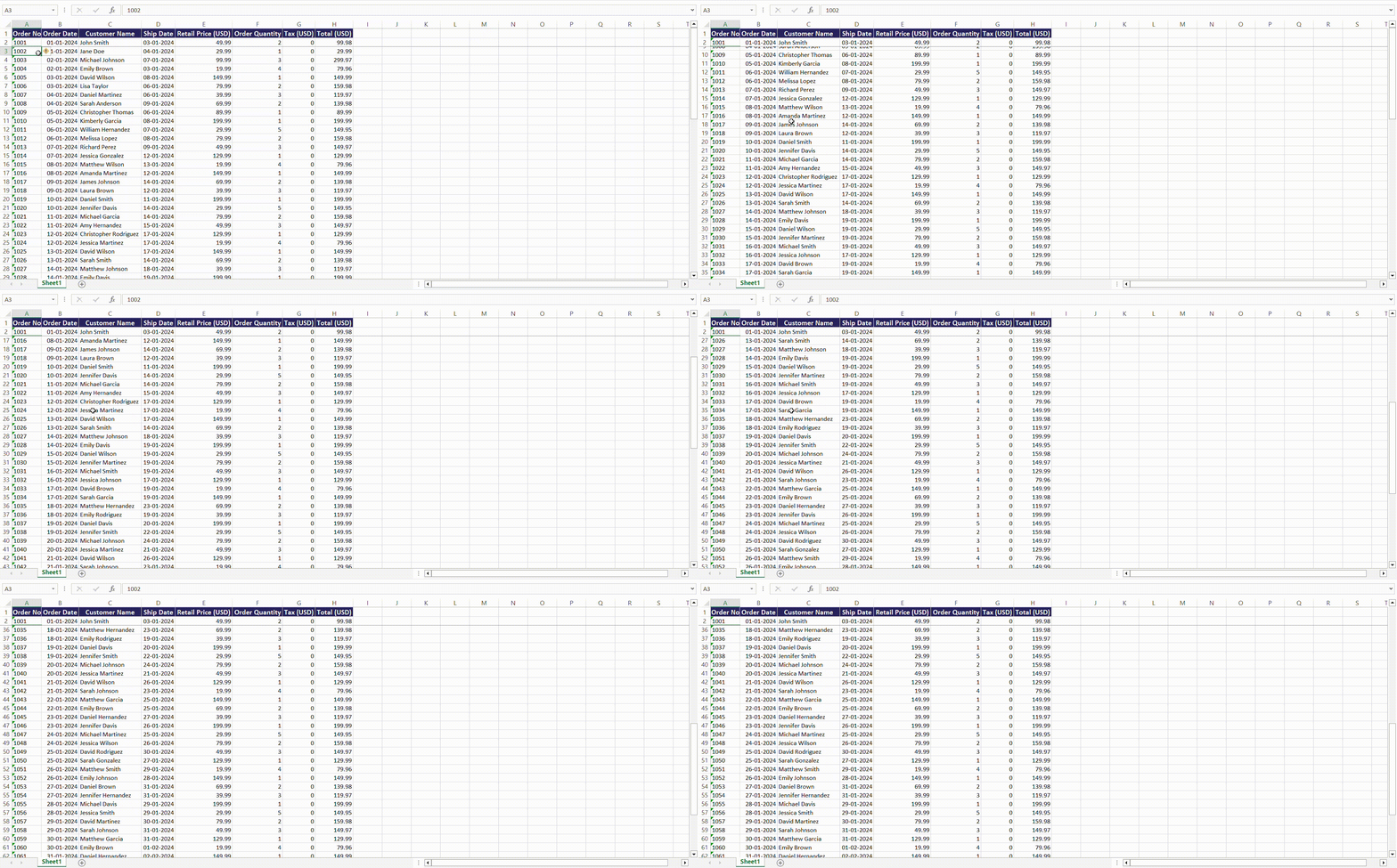
Freeze first two rows in Microsoft Excel is a transformative feature that enhances data navigation and organization. By immobilizing these rows while scrolling through extensive datasets, users can maintain visibility of crucial headers and key information. This introduction outlines a step-by-step guide to leverage Excel’s Freeze Panes feature effectively, ensuring a seamless workflow and improved data analysis experience.

Key Takeaways:

• Excel’s Freeze Panes feature locks rows, ensuring vital information stays visible, enhancing accuracy and workflow efficiency.
• This function locks rows or columns while allowing the rest of the worksheet to move freely, ensuring key information remains visible.
• Essential for extensive spreadsheets where headers vanish during scrolling, aiding data analysis, inventory tracking, and financial modeling.
• Tidy data and ensure headers in rows 1 and 2. Execute row freezing via the “View” tab, anchoring essential rows.

 

Introduction

The Power of Excel in Data Management

Excel isn’t just a tool for crunching numbers; imagine it as a trusted companion for managing a plethora of data. With its robust features and intuitive design, Excel simplifies the organization, analysis, and visualization of your information. Whether you’re balancing budgets, scheduling tasks, or tracking inventory, Excel’s versatility makes data management a breeze.

Why Freezing Rows is a Game Changer

Freezing rows in Excel transforms your scrolling experience. It’s like having road signs along a highway; you never lose sight of where you are. By keeping your headers and important information in view, no matter how far you scroll down, you stay oriented.

This feature is particularly useful in complex spreadsheets with large datasets, where it’s crucial to keep row labels visible for accurate data entry and analysis. Think of it as a strategic anchor, giving you a reference point that helps prevent errors and speeds up your workflow.

 

Understanding the Freeze Panes Feature

What Does ‘Freezing’ Actually Mean in Excel?

In Excel, ‘freezing’ refers to the ability to lock specific rows or columns in place. It’s akin to fixing your headers at the top of the screen while allowing the rest of your worksheet to move freely. This way, as you dive deep into the rows, your headers stay put, and accessible for reference.

It’s like having a header that follows you as you scroll, making it simple to match data to the correct column no matter where you are in the spreadsheet. Freezing panes ensures that you no longer need to memorize or repeatedly scroll up to check what each column represents.

When to Use the Freeze Panes

Consider employing the Freeze Panes feature whenever you work with extensive spreadsheets where headers and key rows disappear off-screen as you scroll. It’s perfect for tasks like:

• Long-Form Data Analysis: Keeping column and row labels visible for consistent referencing.
• Large Inventory Tracking: Ensuring product identifiers remain in view while scrolling through quantities or descriptions.
• Financial Modeling: Maintaining visibility of budget categories or timelines when examining detailed transactions.
• Comparative Data Review: Locking headers in place to compare datasets side-by-side without losing context.
• Dashboard and Reporting: Having titles and key metrics stationary for better readability during presentations or reviews.

In essence, use Freeze Panes to maintain a visual anchor in your spreadsheet, which is invaluable for accuracy and ease of navigation.

 

Step-by-Step Guide to Freezing the First Two Rows

Preparing Your Worksheet

Before you freeze those top rows, a bit of prep will ensure your Excel worksheet is primed for success. Start by tidying up your data; remove any unnecessary spaces or columns that could disrupt the clarity of your headers. Verify that your headers are at the very top rows, ideally in rows 1 and 2, as these are the ones you’ll be locking into place.

Ensure that any filters or sorting options are set up correctly, so they’re not affected by the freeze. It’s a bit like setting the stage before the big performance – the better the preparation, the smoother the show.

Execution of Row Freezing

Now, for the magic act of freezing the first two rows! Here’s what you need to do:

STEP 1: Open your Excel document and make sure you’ve saved all recent changes.

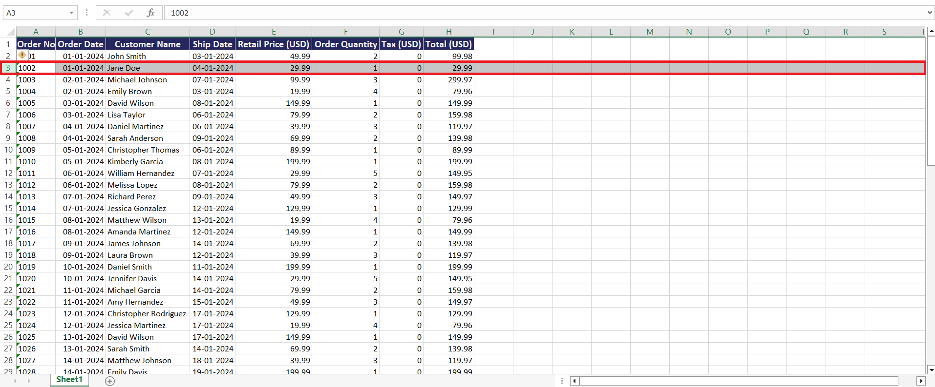
STEP 2: Click on the row number below the ones you want to freeze. To freeze the first two rows, you’ll click on row 3.

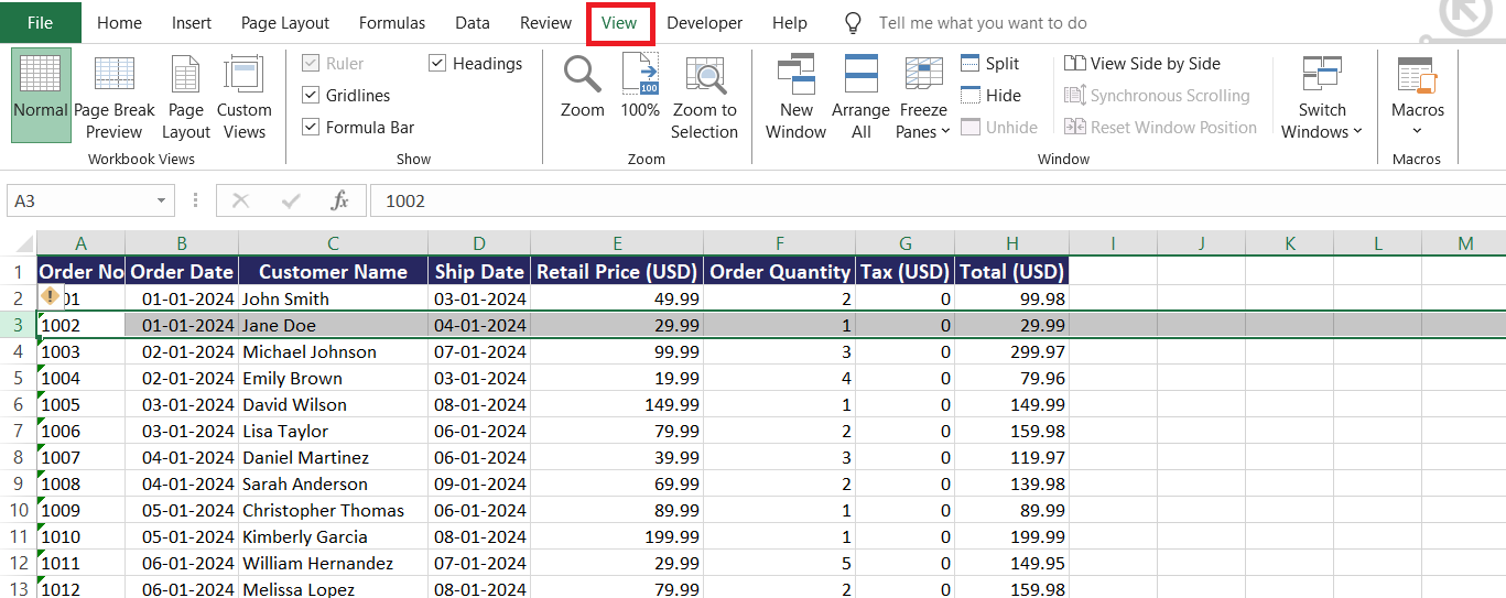
STEP 3: Navigate to the “View” tab on Excel’s ribbon.

STEP 4: Find the “Freeze Panes” button in the “Window” group.

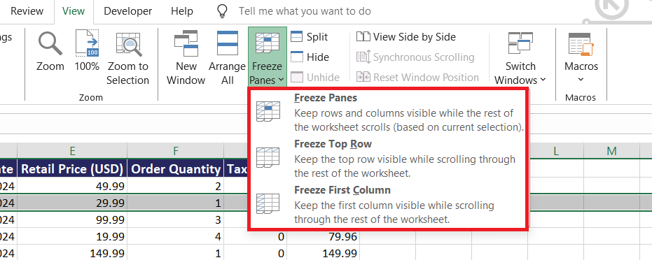
STEP 5: Click “Freeze Panes,” and a drop-down menu will appear.

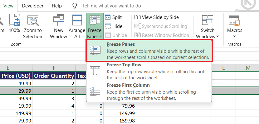
STEP 6: From the options, select “Freeze Top Row” if you only want the very first row frozen. For freezing the first two rows, however, you should choose “Freeze Panes” after clicking on the third row.

STEP 7: As a result, the rows above your selection will stay visible as you scroll down. If you’ve selected row 3, rows 1 and 2 will now be your constant companions in data navigation. It’s a quick process, but the impact on your workflow can be transformative.

 

Tips and Tricks for Managing Frozen Rows

Navigating Through Large Datasets with Ease

With rows neatly frozen, scrolling through large datasets becomes not just manageable, but efficient. You keep your bearings and can perform quick visual cross-referencing or spot-check data against fixed header information, no matter how far down you go.

Another tip for seamless navigation is using keyboard shortcuts; “Ctrl + Arrow” keys let you jump to the edges of your data, while “Page Up” and “Page Down” allow for quicker vertical scrolling. Consider also the use of “Alt + W, F, F” as a shortcut to quickly freeze panes, making the process even more streamlined. With these tools, Excel feels less like a maze and more like a well-organized library.

Ensuring Visibility of Your Top Rows

To keep the top rows in view while perusing through data, freezing those rows is key. Double-check that the correct rows are frozen by scrolling down your worksheet. The frozen rows should remain static and always in sight.

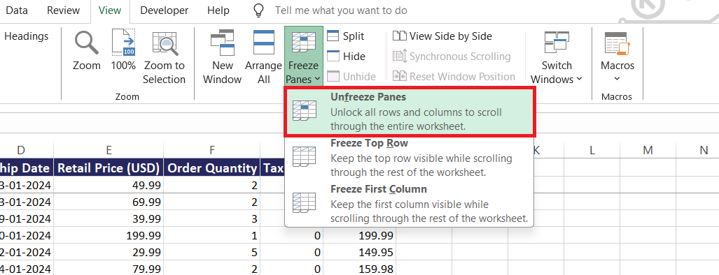
If you need to make adjustments, simply unfreeze the panes by going back to the “View” tab and clicking “Freeze Panes” again, but this time choosing “Unfreeze Panes.”

Readjust as necessary until it’s perfect. Remember, a well-organized spreadsheet with visible headers not only makes data analysis easier but also presents your work in a professional and accessible manner.

 

Troubleshooting Common Issues

Addressing the Disappearing Cell Text Problem

If you’ve ever been puzzled by text seemingly vanishing from a cell as you click on headers, chances are you’ve scrolled too far from the original focus area. To bring everything back into view, simply scroll up or zoom out until you reach the top-left corner of your worksheet (cell A1).

This return to basics realigns your spreadsheet, ensuring you can see and select any cell with confidence. Remember, keeping your headers and key data in sight with frozen panes can prevent this text from disappearing act in the first place.

Fixing Freezing Mishaps

Has freezing gone awry, leaving parts of your worksheet immobilized in all the wrong places? Fear not, fixing freezing mishaps in Excel is a breeze. To reset the situation, simply head to the ‘View’ tab and under ‘Freeze Panes’, select ‘Unfreeze Panes’. This will thaw all your rows and columns, allowing you to start fresh.

When you’re ready to refreeze, remember to select the cell or row right after where you want the freeze to start. Like a good detective, sometimes you have to retrace your steps to get the outcome you’re looking for.

 

FAQs

How to freeze first two rows in Excel?

To freeze the top 2 rows in Excel: Select row 3, then go to the ‘View’ tab, click ‘Freeze Panes’, and choose ‘Freeze Panes’ again from the dropdown. This action locks the first two rows while you scroll.

How do I freeze multiple rows or columns at once?

To freeze multiple rows, select the row below the ones you want to freeze. For columns, select the column right after the ones to freeze. Then, use ‘View’ > ‘Freeze Panes’ > ‘Freeze Panes‘.

Can I freeze both rows and columns simultaneously?

Yes, you can freeze both rows and columns simultaneously in Excel. Click on the cell below and to the right of the rows and columns you want to freeze, then from ‘View’ choose ‘Freeze Panes’ > ‘Freeze Panes’.

Is it possible to freeze panes in Excel Online?

Yes, you can freeze panes in Excel Online too. Just select the desired rows or columns, go to the ‘View’ tab, and then click on ‘Freeze Panes’ to apply the setting.

What if freezing rows are not working properly?

If freezing rows isn’t working, make sure you’re selecting the correct row beneath the ones to freeze. If issues persist, unfreeze panes via ‘View’ > ‘Freeze Panes’ > ‘Unfreeze Panes’, then try again.