The Ultimate Guide to Freeze Panes in Excel

Freeze Panes in Microsoft Excel is a feature that allows users to lock specific rows or columns in place, ensuring they remain visible while scrolling through the rest of the worksheet. This is particularly useful for keeping headers or key data points in view, providing context as you navigate large datasets. By freezing panes, you enhance the usability and readability of your spreadsheets, making data analysis and entry more efficient.

Key Takeaways:

• Enhanced Navigation: Freeze Panes keep specific rows or columns visible while scrolling, maintaining important headers or data in view.
• Simple Access: The Freeze Panes option is easily accessible under the ‘View’ tab in Excel, with multiple options like ‘Freeze Top Row’ and ‘Freeze First Column’.
• Visibility Control: Freezing the top row ensures that critical headers remain visible, improving the ease of navigating and understanding large datasets.
• Stable View: Locking multiple columns by selecting the right adjacent column ensures essential data remains in sight as you scroll horizontally.
• Comprehensive Freezing: Combining frozen rows and columns provides a thorough view of key data, enhancing the efficiency of data analysis and management.

 

Introduction to Mastering Excel Spreadsheets

Encounter the Freeze Panes Feature

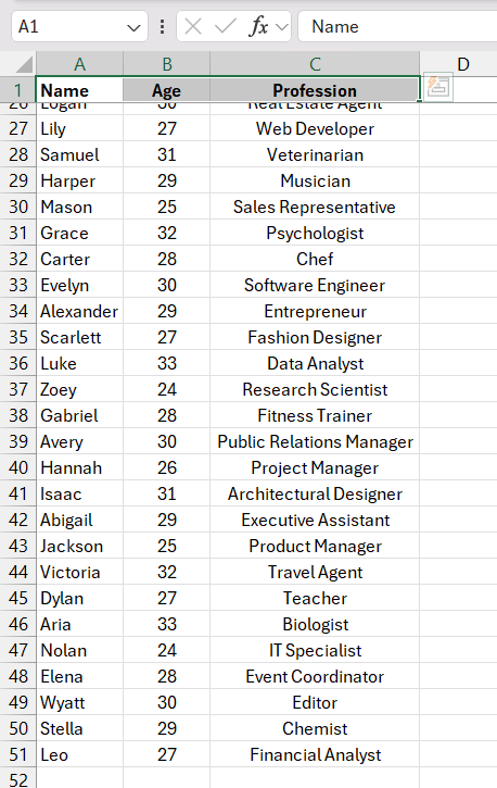
Are you tired of scrolling through your spreadsheet only to lose sight of your headers and forgetting which column represents what? Here comes the Freeze Panes feature to the rescue! Picture this tool as your personal spreadsheet sidekick. It enables you to lock specific rows or columns in place, so no matter how far you scroll down or across, you always have the pivotal information in view.

This feature can be incredibly helpful when dealing with large sets of data and is a game-changer for maintaining context in your spreadsheets.

 

Getting Started with Freeze Panes

Navigating to Freeze Panes Options

Diving into the Freeze Panes options is a breeze once you know where to look. Try the following steps:

STEP 1: Open up your Excel spreadsheet and head to the ‘View’ tab at the top.

STEP 2: From there, glance over to the ‘Window’ group and, voilà, you’ll spot the ‘Freeze Panes’ button, your gateway to locking down your data.

STEP 3: Click it, and you’ll uncover three neat choices: ‘Freeze Panes,’ ‘Freeze Top Row,’ and ‘Freeze First Column.’ Pick the option that suits your spreadsheet’s needs, and you’re all set to scroll through your data without losing sight of your headers.

 

Freezing Top Rows for Enhanced Visibility

Enhancing the visibility of your top rows in Excel is just a few clicks away, which could make all the difference in keeping your work streamlined and stress-free. To put this feature to work –

Select the ‘Freeze Top Row‘ option after clicking ‘Freeze Panes’ under the ‘View’ tab.

This will keep the first row visible as you navigate through the spreadsheet wilderness.

It’s ideal when the top row holds all those critical headers that define each column, so no matter how deep you delve into the data, the top row stays in sight, keeping you on track.

 

Advanced Techniques with Freeze Panes

Locking Multiple Columns for Stability

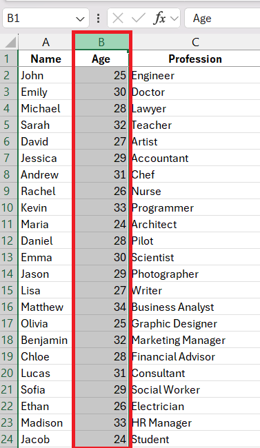
Locking multiple columns is a stable move for those larger spreadsheets where critical label columns need to stay in the foreground of your work. To achieve this stability –

STEP 1: You need to select the column to the right of the columns that need to be frozen.

STEP 2: After making the selection, they would then navigate to the ‘View’ tab, engage the ‘Freeze Panes’ drop-down, and select ‘Freeze Panes’ again.

STEP 3: The result is a steadfast set of columns on the left, anchored securely as you explore the data bounty to the right.

It’s a remarkably simple way to maintain a steady frame of reference in your burgeoning spreadsheet.

 

Combining Frozen Rows and Columns for Comprehensive Views

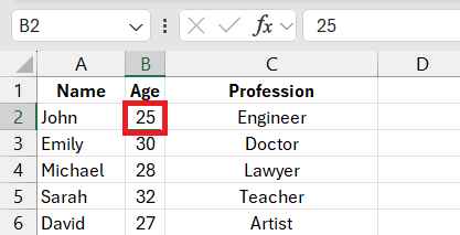
For a truly comprehensive view that captures both your pivotal rows and columns, you can combine the powers of both freezing techniques. The magic lies in choosing the right cell before activating the Freeze Panes. Imagine you want to freeze both the first two columns and the top three rows.

You would select cell B2—the cell below and to the right of the columns and rows you wish to freeze.

From there, journey to the ‘View’ tab, summon the ‘Freeze Panes’ command, and voilà – your spreadsheet now holds both rows and columns static, providing an unwavering view of your key data as you navigate.

This level of control ensures a seamless analysis experience, where no data point goes unnoticed, no matter where it is on the grid. It’s perfect when you have both row and column headings that are crucial to understanding the entirety of your data.

 

FAQ: Mastering Freeze Panes in Excel

What is freeze pane?

Freeze Pane is a handy Excel function that keeps selected rows or columns visible while you scroll through your spreadsheet. It’s perfect for maintaining a constant reference point, particularly with headers that label data columns or rows. Think of it as a way to keep your bearings in a sea of numbers and text, ensuring you always have the context you need without constantly scrolling back and forth.

How do I freeze certain panes in Excel?

Freezing panes in Excel is straightforward. Click on the cell to the right and below the rows and columns you’d like to freeze. Afterward, navigate to the ‘View’ tab, click ‘Freeze Panes,’ and once more select ‘Freeze Panes’ from the dropdown menu. Rows above and columns to the left of the selected cell will remain visible as you navigate through your spreadsheet.

What is the shortcut for Freeze panes in Excel?

To quickly freeze panes in Excel without navigating through the menus, you can use a keyboard shortcut. Initially, position your cursor in the cell where you intend to begin the freeze. Then press ‘ALT + W + F’. This will instantly apply the Freeze Panes feature right from your keyboard, streamlining your workflow. Additionally, if you want to freeze the top row or first column specifically, use ‘ALT + W + R’ for the row, or ‘ALT + W + C’ for the column.

How Do I Freeze More than One Rows or Columns Simultaneously?

If you want to freeze the first four rows and the first three columns, place your cursor in cell D5. This is because Excel freezes rows and columns up to the one before your selected cell. Next, go to the ‘View’ tab, click on ‘Freeze Panes,’ and select ‘Freeze Panes’ from the dropdown menu. This will lock both the specified rows and columns in place, ensuring they remain visible as you navigate through your spreadsheet. Remember, selecting the correct cell is key; once you do that, you’re set.

Can I Freeze Panes for Only Specific Cells in My Spreadsheet?

Unfortunately, Excel doesn’t allow you to freeze individual cells. Freeze Panes works for entire rows or columns. If you want to keep select cells visible, you’ll need to freeze the rows and columns that contain those cells. Alternatively, consider using features like Split Panes or adjusting your layout to keep critical data in view as you maneuver through your spreadsheet.