Maximizing Efficiency with Freeze Rows in Excel

Freezing rows in Microsoft Excel is a handy feature that keeps your headings visible as you navigate through lengthy spreadsheets. This function particularly enhances the readability and manageability of large datasets by allowing users to lock specific rows at the top of the worksheet. This functionality is particularly beneficial when tracking or comparing information across different sections of the worksheet.

Key Takeaways

• To freeze rows or columns in Excel, select the one you want to keep visible and click “Freeze Panes” from the “View” tab.
• Freezing panes keep selected rows and/or columns in view while scrolling through your worksheet.
• Splitting panes, different from freezing, divides your worksheet so you can scroll different sections independently.
• Use the “Freeze Panes” command for locking specific rows or columns to make navigating large datasets easier.

 

Introduction to Freezing Rows in Excel

Why Visibility Matters When Working with Large Spreadsheets

When working with large spreadsheets, it’s crucial to keep key data points within sight. The top rows often contain headers or important figures that guide the rest of your data entries. Freezing these Rows in Excel ensures that, no matter how much you scroll, the information you need to make accurate comparisons or decisions remains ever-present. The benefits are crystal clear – fewer mistakes and increased efficiency.

The Basics of Locking Rows in Excel for Ease of Data Analysis

Locking rows, commonly known as “freezing,” allows for unfaltering data visibility and eases the process of data analysis. When rows are frozen, they anchor your most pivotal data — like headers or summary info — making sure these remain constant at the top of your screen while you delve into the depths of your data below. It’s a simple feature, but it transforms your workflow, granting you a persistent frame of reference.

 

Step-by-Step Instructions for Freezing Rows

How to Freeze the Top Row in Your Spreadsheet

Freezing the top row of your spreadsheet is a swift and straightforward task that enhances your ability to stay oriented within your data. Here’s how you can freeze rows in Excel –

STEP 1: Open your spreadsheet and ensure the top row with your headers or titles is in view.

STEP 2: Go to the “View” tab located in Excel’s ribbon.

STEP 3: Click on “Freeze Panes” in the Window group.

STEP 4: Select “Freeze Top Row” from the dropdown menu.

Now, as you scroll down your spreadsheet, your top row remains visible, serving as a static guide amidst a sea of ever-changing data.

Remember, this process locks the first row that is visible under your column labels. That means it’s crucial to have your headers right at the top before initiating the freeze.

Techniques for Freezing Multiple Rows for Better Data Management

For those who manage extensive spreadsheets, freezing multiple rows is a game-changer. It facilitates the monitoring of various headings or key figures spanning several rows at the top of your sheet. Let’s freeze:

STEP 1: Decide which rows you need to keep in view.

STEP 2: Click on the cell immediately below the last row you want to freeze.

STEP 3: Head to the “View” tab in Excel’s ribbon.

STEP 4: Choose “Freeze Panes” in the Window group.

STEP 5: Click “Freeze Panes” in the dropdown menu.

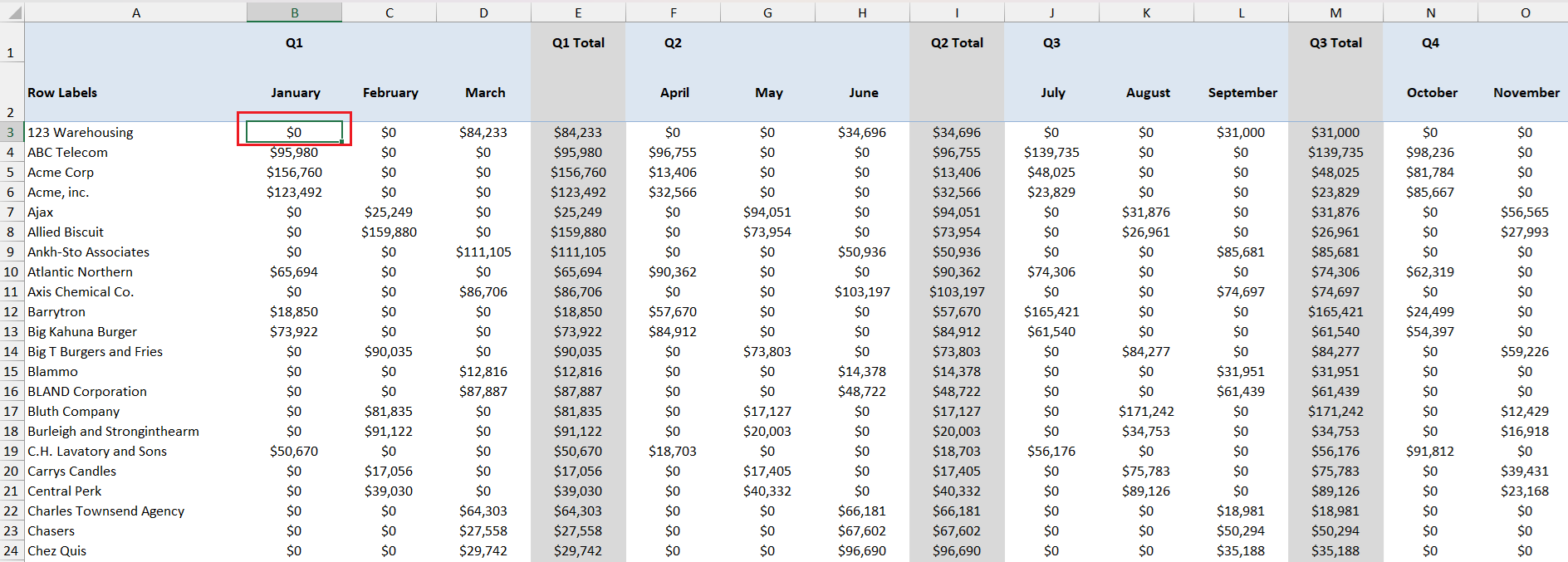
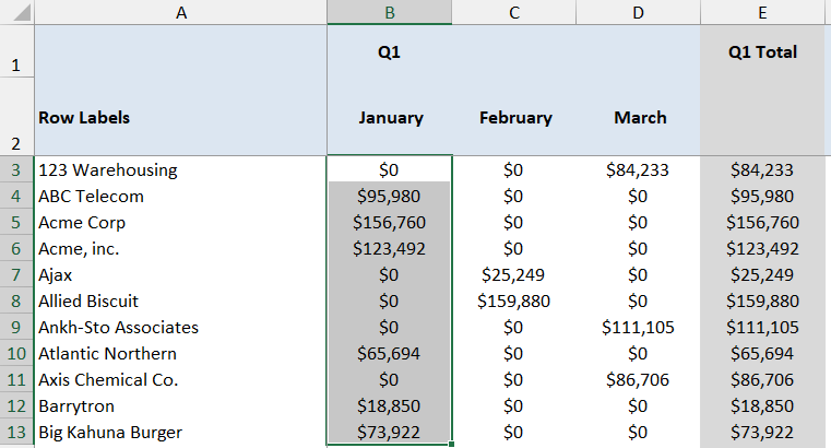
This action freezes everything above your selected cell. For example, click cell B3 to freeze the first two rows and one column. A thicker line appears below the frozen section, serving as a visual cue.

Perfecting this technique means that you never lose sight of crucial data while navigating through long lists or comprehensive data sets.

 

Optimizing Your Excel Workflow

Best Practices when Using Freezing Features

When utilizing Excel’s freezing features, adopting a set of best practices can enhance your data management experience. Here’s what you should keep in mind:

• Always review your dataset before applying the freeze, ensuring that the rows or columns you lock in place contain the necessary reference points.
• Combine freezing with other Excel features like “Sort” and “Filter” to manage large datasets more efficiently.

• Avoid freezing too many rows or columns, as this can limit the visible unfrozen area of your worksheet.
• If you collaborate with others, communicate which rows or columns are frozen, as this will affect how associates navigate the spreadsheet.

 

Troubleshooting Common Issues When Freezing Rows

Even seasoned Excel users can encounter issues when freezing rows. If you’re having trouble, consider these common pitfalls and solutions:

• Frozen Rows Aren’t Locked in Place: Check that you’ve selected the correct row below the ones you wish to freeze. Also, make sure you’ve clicked “Freeze Panes” and not accidentally “Freeze Top Row” or “Freeze First Column.”
• Freezing the Wrong Rows: To fix this, first “Unfreeze Panes” and then freeze the correct rows following the steps provided previously. Always double-check which cell you’ve selected before you click to freeze.
• Unable to See Frozen Rows While Scrolling: If your top rows disappear, it might be because your workbook is in “Split” view rather than “Freeze Panes.” Double-check that you’ve used the correct option.
• Lost Scrollability: If you’ve frozen too many rows, you might find yourself unable to scroll up and down effectively. Unfreeze some rows to regain navigation control.

When troubleshooting, also make sure to check if your workbook is in “Page Layout”, as freezing panes only works in “Normal” mode. If problems persist, restarting Excel can refresh settings that might have been mistakenly altered.

 

Advanced Tips for Excel Users

Customizing Scroll Settings for Enhanced Navigation

To fine-tune your navigation in Excel, customizing your scroll settings can significantly improve your workflow. Here are some ways to tailor your scrolling experience:

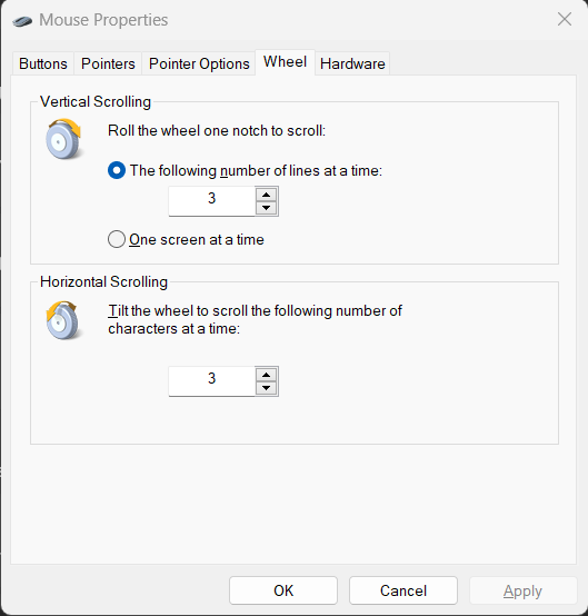
• Scroll Direction: Toggle between horizontal and vertical scrolling to suit your data layout. Change this in your mouse or touchpad settings outside of Excel.

• Scroll Speed: Adjust the scroll speed to match your pace. This is especially useful when scanning through long datasets.

By tailoring these settings, navigation becomes more intuitive and less of a strain, allowing you to focus more on analysis and less on the mechanics of getting around your spreadsheet.

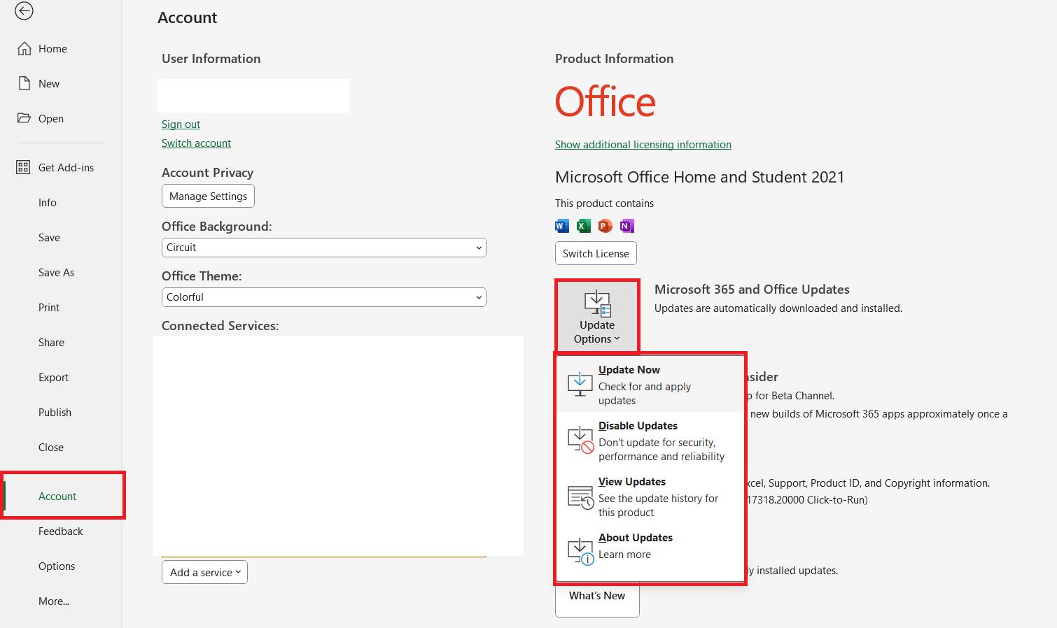
Remember to update your Excel to the latest version to enjoy the full benefits, including the Smooth Scrolling feature, which was recently updated on December 15, 2022, for all users on monthly “production” updates. To check for updates, go to “File” > “Account” > “Update Options”.

 

Protecting Frozen Rows from Unintended Edits

Protecting your frozen rows from unintended edits is crucial, especially when sharing your Excel file with others. Here’s how to safeguard your data:

STEP 1: Select the cells or rows you want to protect.

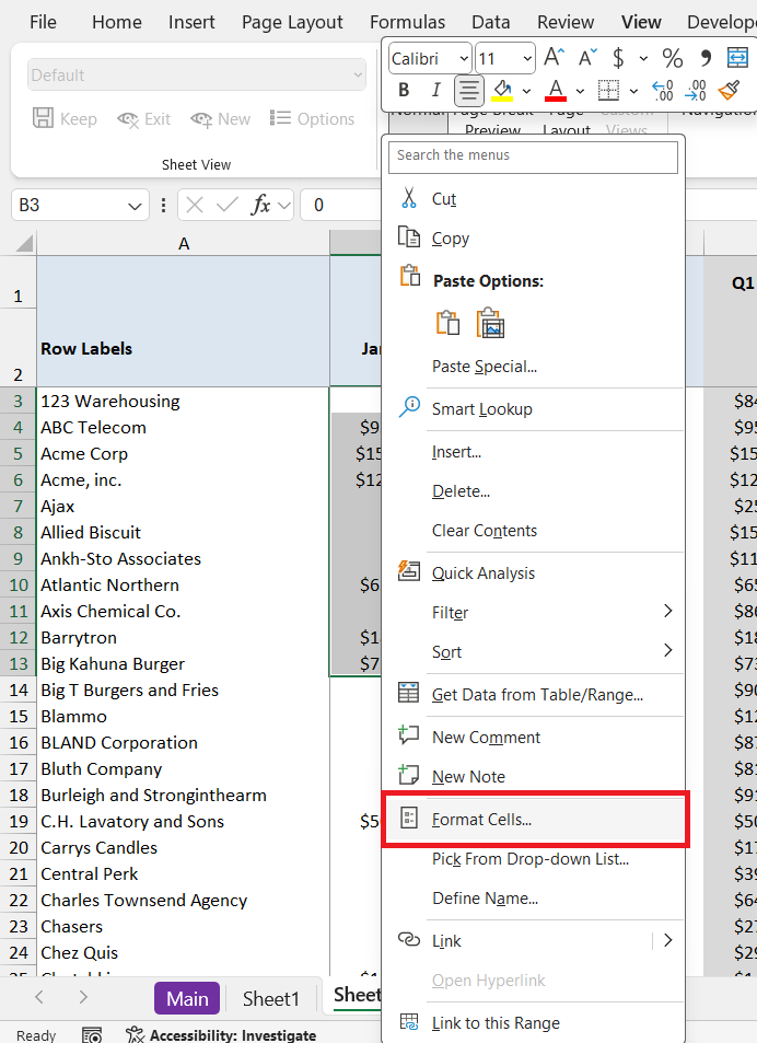
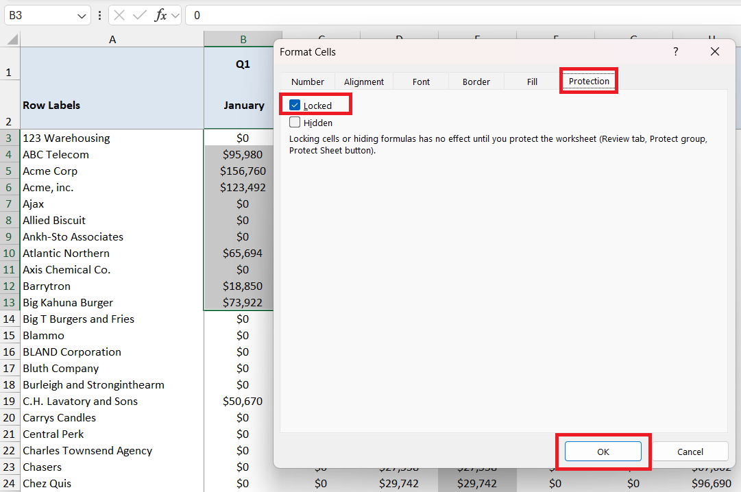
STEP 2: Right-click and select “Format Cells” from the dropdown.

STEP 3: In the “Protection” tab, ensure “Locked” is checked. This option is on by default.

STEP 4: Close the dialogue box and then click on “Review” in the ribbon.

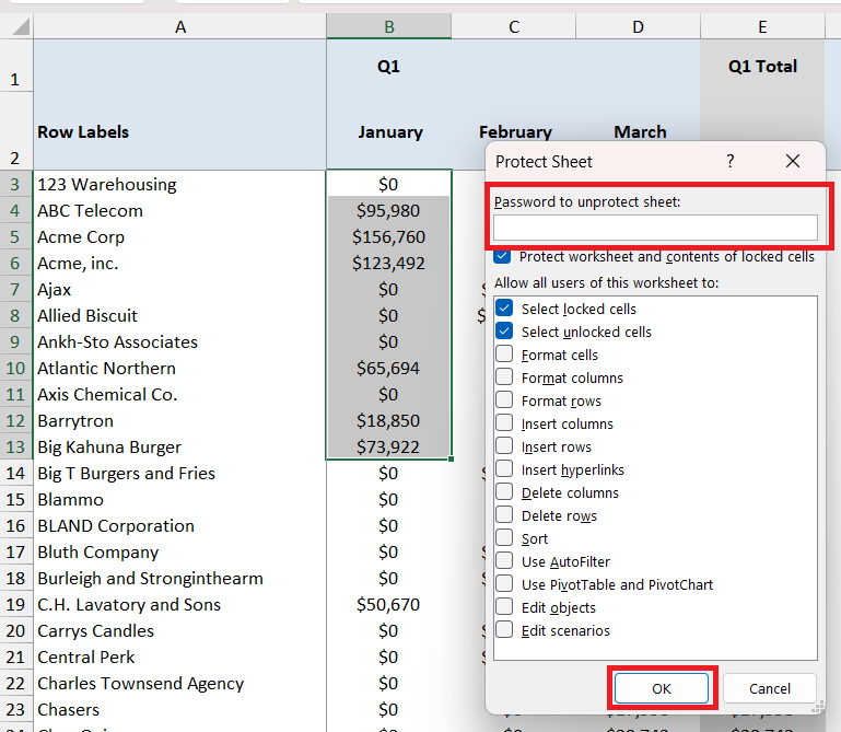
STEP 5: Click “Protect Sheet” to set up a password and select actions that you want to allow.

This locks the selected cells, preventing any modifications unless the sheet is unprotected. Especially useful for rows with formulas or critical headers, it adds an extra layer of security, ensuring that the integrity of your data is maintained.

 

Collaborative Excel Workspaces

Maintaining Data Integrity with Locked Rows

Ensuring the integrity of your data is paramount in a collaborative workspace. Locked rows serve as a steadfast reference point, critical when multiple users access the same document. Here’s how locked rows help:

• They keep formulae intact, preventing accidental changes that could corrupt data.
• Consistency is maintained as headers and other important information stay in view for all users.
• Changes can be traced more easily, since the fixed data will likely contain clues as to where an inconsistency may have been introduced.

 

Sharing Tips for Teams Using Frozen Rows in Excel

Teams can make the most out of Excel’s freeze functionality when collaborating on spreadsheets by following a few shared practices:

• Communicate Clearly: Always inform your team when you freeze rows—or make any significant changes—to prevent confusion during data analysis.
• Standardize Practices: Develop a team standard for when and how to use frozen rows, ensuring consistency across different documents and users.
• Use Named Ranges: For sections that are frequently frozen, define and use named ranges, making it easier for everyone to understand what section is being referred to.

These shared habits uphold data visibility and foster a collaborative environment where the spreadsheet’s functionality is used efficiently and effectively.

 

Beyond Basic Freezing: Other Navigation Shortcuts

Split Panes for Comparative Data Analysis

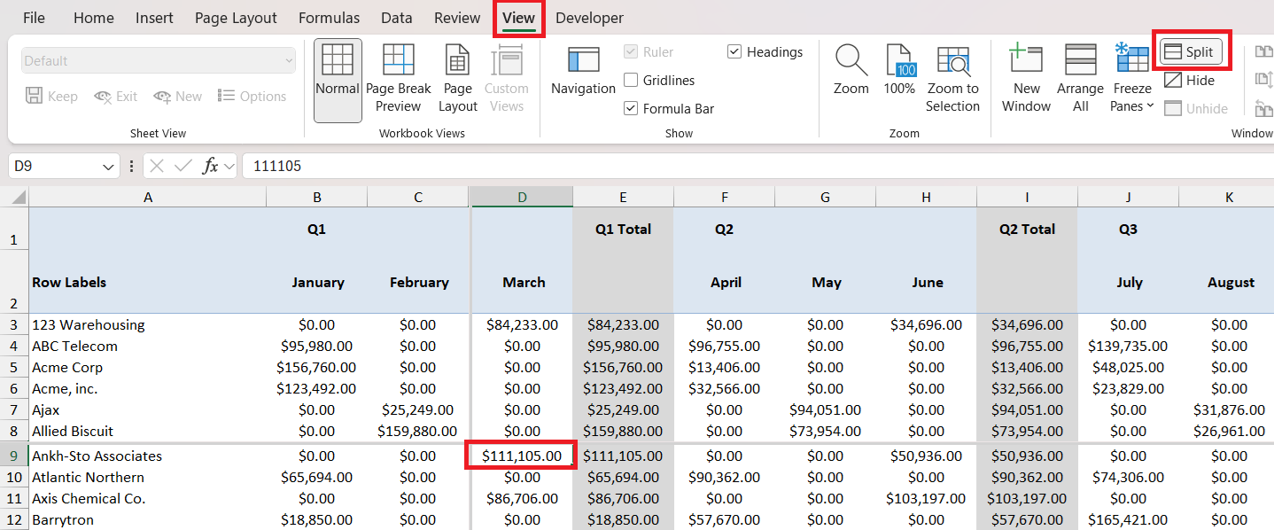
Splitting panes in Excel offers a dynamic way to compare different sections of your data simultaneously. Unlike freezing rows or columns, splitting divides your screen into separate scrollable areas. Here’s why it’s beneficial:

• Targeted Comparison: Easily compare distant rows or columns without incessant scrolling.
• Customized Viewpoints: Tailor your screen to show exactly what you need, side by side or above and below.

To split panes, simply select a cell below or to the right of where you want the split and then go to “View” > “Window” > “Split.” You’ll now have either two or four independently scrollable areas, depending on whether you split both ways.

 

Unlocking Rows and Columns: Reversal Techniques

Sometimes you might need to reverse the freezing process to regain the full view of your Excel sheet. Here’s how to unfreeze, or unlock, your rows and columns:

STEP 1: Navigate to the “View” tab on the Excel ribbon.

STEP 2: Go to the “Window” group and click on “Unfreeze Panes.”

STEP 3: This action will unlock any frozen sections, rows, or columns on your current worksheet.

It’s a quick and seamless process that restores your scrolling ability to its original state, giving you a clean slate for tasks that require a complete, unobstructed overview of your data. This function is particularly useful when transitioning from data entry to final formatting or when adjusting the layout of your dataset for presentation purposes in Microsoft Excel. Remember to communicate these changes to your team to maintain collaborative efficiency.

 

FAQ: Navigating the Freeze Function in Excel

What’s the Difference Between Freezing Rows and Splitting Panes?

Freezing rows keeps specific rows or columns in place as you scroll through the rest of your worksheet. It’s perfect for keeping headers visible. Splitting panes, meanwhile, divide your Excel window into separate scrollable sections, so you can view and scroll through different parts of your spreadsheet simultaneously. Use freezing for constant visibility and splitting when comparing different dataset areas.

How Can I Freeze Rows and Columns at the Same Time?

To freeze rows and columns simultaneously in Excel, select the cell that is below and to the right of the rows and columns you want to lock. Then, go to the “View” tab, click “Freeze Panes,” and choose “Freeze Panes” from the list. This will lock both the rows above and the columns to the left of your selected cell, keeping them visible as you scroll down or across your worksheet. Give it a try to keep important headers and labels always in sight.

Can I Still Edit Data in Frozen Rows?

Yes, you can still edit data in frozen rows. Freezing panes in Excel doesn’t prevent editing; it simply keeps certain rows or columns in view while you scroll through the rest of your data. Feel free to click on any cell within the frozen sections to make changes as needed. However, remember to exercise caution to maintain data integrity, especially when working with formulas or shared documents.

Why Are My Frozen Rows Not Working, and How Can I Fix It?

If your frozen rows aren’t working, first ensure you’re not in cell editing mode; press Enter or Esc to exit. Next, check if your worksheet is protected and remove protection if needed. Confirm you’ve selected the row below the ones you wish to freeze. Also, make sure you’re in “Normal” view, as freezing doesn’t apply to other layout views. Review these points, make adjustments as necessary, and your frozen rows should work correctly. If you continue to face issues, consider restarting Excel to reset any inadvertent changes to your settings.