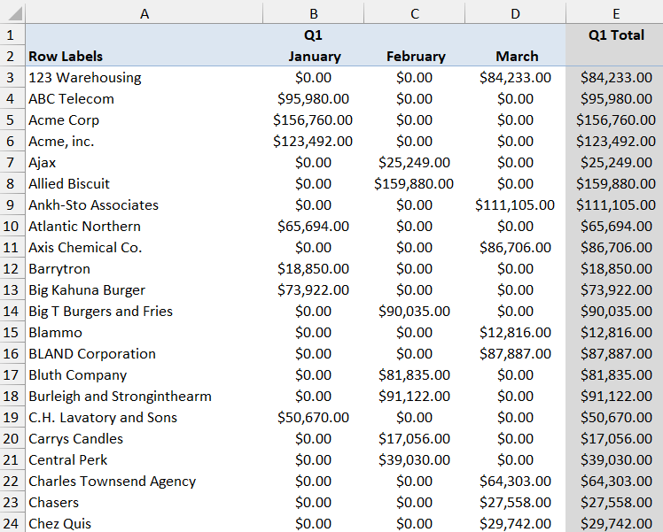
Freezing the second row in Microsoft Excel ensures that it remains visible as you scroll through long datasets, keeping key information at the top of your screen. This feature is particularly handy for maintaining header visibility or comparing values across different parts of your spreadsheet. Here’s a quick guide on how to freeze second row into place for easier navigation and data analysis.
Key Takeaways
- To freeze the second row in Excel using the View tab, first select the third row, then select the View tab and click on ‘Freeze Panes‘ followed by ‘Freeze Panes’ again from the dropdown.
- Keyboard shortcuts can expedite the process; after selecting the third row, press Alt+W, F, F to freeze the second row instantly.
- Utilize the Quick Access Toolbar for efficiency; add the ‘Freeze Panes’ command to the toolbar, highlight the third row, and click the newly added freeze button to lock the second row.
- For regular users of this function, creating a macro can automate the freezing process; record a macro of you freezing the second row and assign it a shortcut or button for future one-click use.
Understanding Freezing vs. Locking Cells
Why Focus on the Second Row?
Sometimes, the first row of your Excel spreadsheet isn’t the header; it could be a title, an image, or some introductory text. When this happens, the header—that indispensable key to understanding your data rows—could be situated on the second row.
By freezing the second row, you make sure your headers stay in place as you navigate through your sea of data, granting you continuous context and making comparisons a breeze. Keeping this crucial information visible at all times can significantly ease data management tasks, especially in larger spreadsheets.
Freeze Second Row – Simplified
STEP 1: Navigate to Your Desired Worksheet
Before anything else, make sure you’re on the right track by opening the Excel workbook containing the relevant data. Within the workbook, click on the specific worksheet tab at the bottom where you wish to freeze second row. This initial step is important—you want to ensure that you’re not making changes to the wrong sheet, which could cause confusion or the loss of time correcting mistakes.
STEP 2: Select the Correct Cell to Activate Freeze Panes
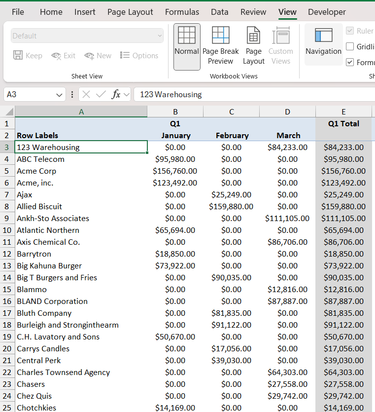
Now that you’re in the correct worksheet, it’s time to select the appropriate cell to activate the freeze panes feature. To freeze second row, choose the cell located in the third row directly beneath the row you intend to freeze. For this case, this would be cell A3. By selecting this cell, you’re indicating to Excel that you wish to freeze everything above this point, meaning the first and second rows.
STEP 3: Implement the Freeze Panes Feature
Great, you’ve selected cell A3. Now let’s engage the freeze! Head up to the View tab in the Excel ribbon—this is your control tower for what you see on your screen. From there, locate the ‘Window’ group and click on ‘Freeze Panes.’ A small drop-down will appear; select ‘Freeze Panes’ again from the options listed.
And just like that, boom!
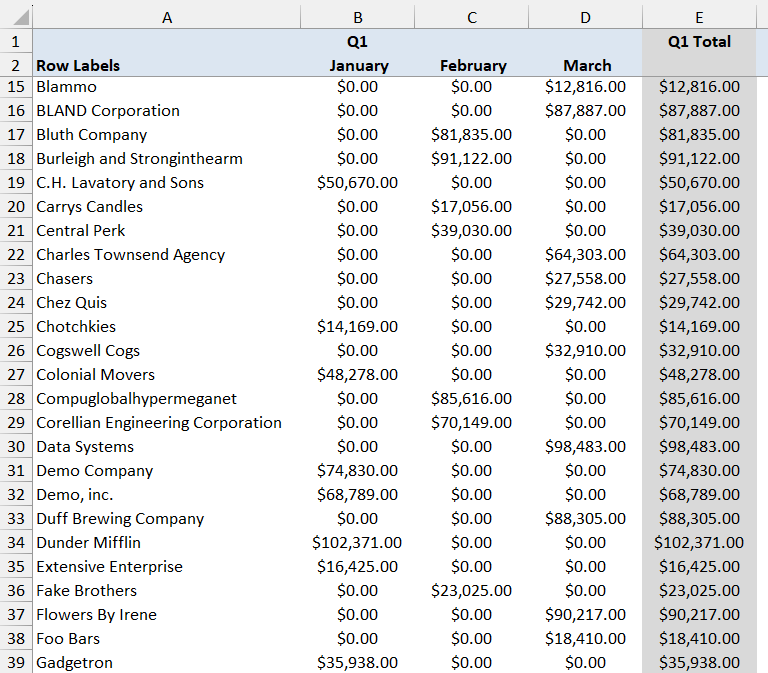
You’ve anchored the second row. Scroll down or across your sheet to see your work in action; rows one and two remain steadfast at the top while the rest of your data freely moves.
Practical Applications for Frozen Rows
Improved Data Analysis with Stationary Headers
With the second row frozen in place, Excel transforms into a more powerful tool for data analysis. As you venture down the rabbit hole of your dataset, the stationary headers serve as a constant reference, eliminating the need to scroll up repeatedly to recall which column represents which data point. This simple yet effective tweak can significantly improve efficiency, reduce errors, and keep your analysis process smooth and uninterrupted.
Keeping Key Information Always in Sight
The decision to keep the second row visible at all times is a game-changer for maintaining a high degree of situational awareness while working through extensive spreadsheets. Whether it’s a pivotal set of category names, key metrics, or critical date lines, freezing the second row ensures that relevant information remains in your line of sight. This constant visual presence helps prevent misinterpretation of data, promotes accuracy in your work, and enables quicker cross-referencing, especially in dynamically updated sheets or when filters are applied.
Tips and Tricks for a Smooth Experience
Shortcuts for Quick Freezing
Speed up your workflow with a few handy keyboard shortcuts! To instantly freeze second row, use the Alt + W + F + F. Here’s how you do it: once you’ve selected the cell below the row you want to freeze (for the second row, that’s A3), simply press and release the ‘Alt’ key, followed by ‘W’, then ‘F’, and ‘F’ again. Excel swiftly locks the rows in place, giving you a quick freezing action without the mouse gymnastics.
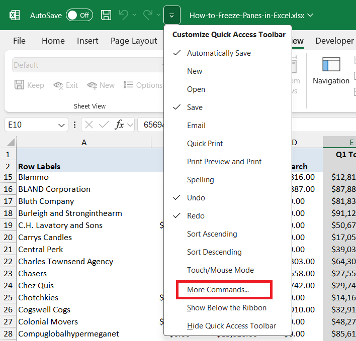
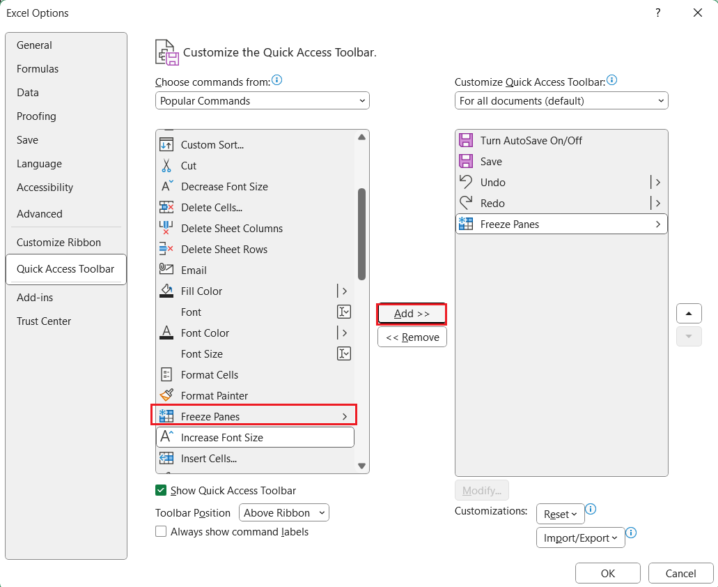
For power users frequently adjusting their view, customizing the Quick Access Toolbar to include the Freeze Panes command can save loads of time. Here are the steps to add the Freeze Panes command to the Quick Access Toolbar in Excel:
STEP 1: Click the down arrow at the very top of the Excel window to open the Quick Access Toolbar’s customization dropdown menu and select “More Commands” from the dropdown menu to open the Excel Options dialog box.
STEP 2: In the Excel Options dialog box, Scroll through the list of commands until you find “Freeze Panes”. Click to highlight “Freeze Panes,” then select “Add” to move the command to the list of tools in the Quick Access Toolbar.
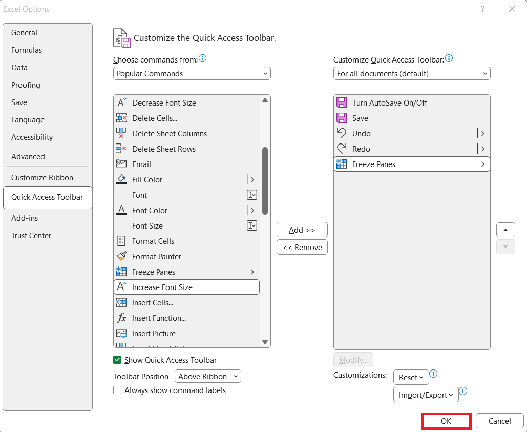
STEP 3: Once “Freeze Panes” is added to the right-hand side list, click “OK” to finalize your changes and close the Excel Options dialog box.
Your Quick Access Toolbar will now have the Freeze Panes command for easy access whenever you need to freeze rows or columns in your spreadsheets.
This way, you get a ‘magic freeze button’ right there for your convenience.
Best Practices When Working with Large Datasets
When you are tackling the Goliath of large datasets, every slingshot counts. Keep your Excel environment efficient and your mind clear by embracing these best practices:
- Limit Frozen Columns: Practice restraint and freeze only essential columns; less is more for clarity and performance.
- Use Headers and Filters: Headers give structure; filters swiftly refine. Marrying the two helps navigate the data.
- Optimize Your View: Lean on Excel’s ‘View Side by Side’ and customizable zoom features for a tailored data vision.
- Know When To Unfreeze: Routine unfreezing refreshes your perspective and prevents tunnel vision.
By integrating these methods, you can strut through data jungles with deft agility and emerge with insights, not just information.
Troubleshooting Common Problems
What to Do When Freeze Panes Is Not Working
Encountering a snag with the ‘Freeze Panes’ feature? Take these quick steps to problem-solve:
- Exit Cell Editing Mode: If you’re typing or editing, ‘Freeze Panes’ won’t engage. Hit ‘Enter’ or ‘Esc’ to exit.
- Check Workbook Protection: ‘Freeze Panes’ may hide under lock and key. Unprotect your sheet to access the feature.
Still frozen in the unfreezing predicament? Do a quick review of your Excel version‘s compatibility or consider restarting the program to give it a gentle nudge.
How to Unfreeze Rows
As you continue with your tasks, there might come a moment when you need to thaw your spreadsheet and unfreeze those rows. This process is as simple as it was to freeze them:
STEP 1: Go to the ‘View’ tab along the top of your Excel window.
STEP 2: Locate and click on ‘Freeze Panes’ within the Window group.
STEP 3: From the drop-down menu that appears, select ‘Unfreeze Panes’.
That’s it! You’re back to a fully scrollable sheet. Use this feature with flexibility—freeze when you need stability, and unfreeze to regain the full view.
Enhancing Productivity with Advanced Techniques
Automating Row Freezing with VBA Macros
Automating row freezing with VBA macros is like having a personal Excel wizard at your command. VBA (Visual Basic for Applications) allows you to create small programs that perform tasks within Excel, saving you time and effort. For instance, by running a simple macro, you can freeze second row across multiple sheets or workbooks with a single command:
To use this macro, press Alt+F11 to open the Visual Basic Editor, insert a new module, paste the code, and hit F5 to run it.
With VBA, your repetitive tasks melt away, leaving you to focus on the analysis that matters.
Customizing Freeze Panes for Optimal User Experience
Excel offers you the reins to customize the freeze panes to fit your unique workflow. If freezing the second row is just the starting point, you can also freeze columns or create a combination of frozen rows and columns. To do this:
- For Columns: Click on the cell to the right of the column you want to freeze. Then, select ‘Freeze Panes’. This keeps your selected column and all columns to its left stationary.
- For Both: Select the cell situated beneath and to the right of the rows and columns you wish to freeze. Freeze from there, and now both row and column headers are locked in place during scrolling.
You can cater the freeze panes feature to support how you process your data. Whether it’s analyzing customer data, tracking project timelines, or comparing financial reports, customize your freezing for a data experience that’s tailored just for you.
FAQs
Can I Freeze Multiple Rows at Once?
Absolutely! In Excel, you can freeze multiple rows at the same time. Simply select the row right under the last row you want to freeze and then follow the standard freeze panes process. So, if you want to freeze the first five rows, select row 6 and use the freeze panes functionality.
How Do I Keep Columns Visible While Scrolling?
To keep columns visible while you scroll, click on the cell to the right of the column you wish to remain on-screen.
Next, navigate to the ‘View’ tab, click on ‘Freeze Panes,’ and select ‘Freeze Panes’ again. This action will lock the selected column and all columns to its left.
What’s the Difference Between Splitting and Freezing Panes?
Splitting divides your Excel window into separate panes that can be scrolled independently, while freezing keeps selected rows and columns static as you scroll through the rest of your worksheet. Splitting is like opening new viewing windows within the same sheet, whereas freezing is like fixing parts of the sheet in place.
How Can I Unfreeze the Second Row Only?
To unfreeze just the second row, you’ll need to unfreeze all panes first and then re-freeze only what you need. Go to ‘View’ > ‘Freeze Panes’ > select ‘Unfreeze Panes’. Then, if you need to keep the first row frozen, simply select the cell in the second row and refreeze.
John Michaloudis is a former accountant and finance analyst at General Electric, a Microsoft MVP since 2020, an Amazon #1 bestselling author of 4 Microsoft Excel books and teacher of Microsoft Excel & Office over at his flagship MyExcelOnline Academy Online Course.


