In our previous post, we were able to Group by Month using Pivot Tables. Let us take it up another notch, and group it by Half Years!
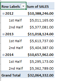
In the example below I show you how to get the Sales Grouped by Half Years: January to June and July to December
STEP 1: Insert a new Pivot table by clicking on your data and going to Insert > Pivot Table > New Worksheet or Existing Worksheet
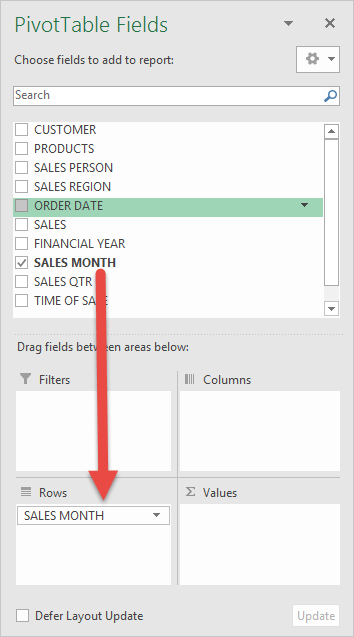
STEP 2: In the ROWS section put in the Sales Month field.
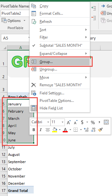
STEP 3: Highlight the first 6 months (January – June). Right click on a row in your Pivot Table and select Group
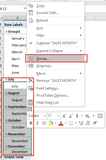
STEP 4: Highlight the next 6 months (July – December). Right click on a row in your Pivot Table and select Group
STEP 5: Rename the groups to make it more readable.
Rename “Group1”to “1st Half”, then rename “Group2” to “2nd Half”.
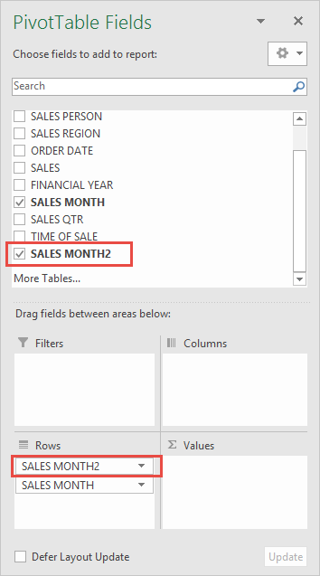
Notice that a new field Sales Month2 was introduced. This contains our new half-year groupings.
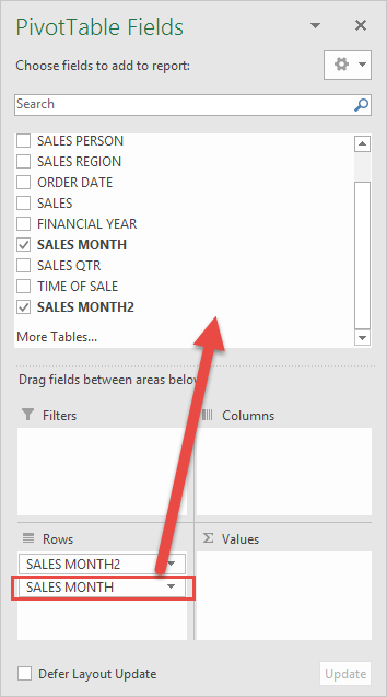
STEP 6: We do not need the Sales Month anymore. Delete Sales Month by dragging it back to the Field List.
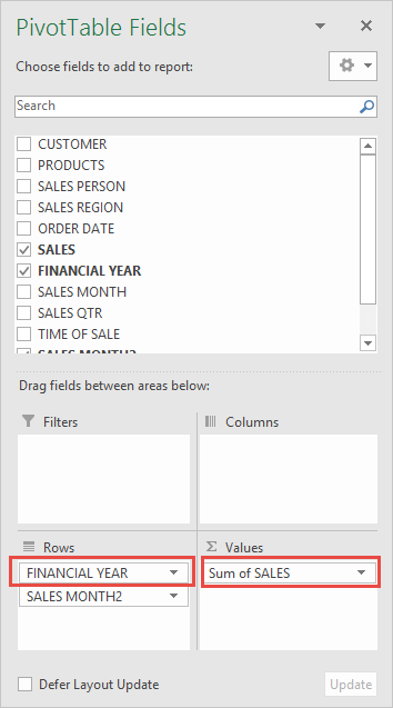
STEP 7: In the VALUES area put in the Sales field. This will get the total of the Sales for each half-year range you have defined.
In the ROWS area put in the Financial Year field on top of the Sales Month2 field:
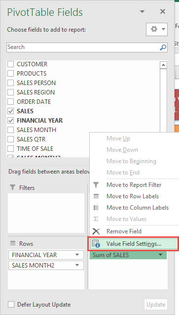
STEP 8: Click the Sum of SALES and select Value Field Settings
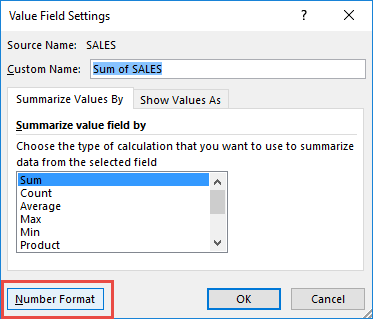
STEP 9: Select Number Format
STEP 10: Select Currency. Click OK.
You now have your total sales for each half-year period!

Bryan
Bryan Hong is an IT Software Developer for more than 10 years and has the following certifications: Microsoft Certified Professional Developer (MCPD): Web Developer, Microsoft Certified Technology Specialist (MCTS): Windows Applications, Microsoft Certified Systems Engineer (MCSE) and Microsoft Certified Systems Administrator (MCSA).
He is also an Amazon #1 bestselling author of 4 Microsoft Excel books and a teacher of Microsoft Excel & Office at the MyExecelOnline Academy Online Course.


