2 Quick Ways to Group Time in Excel Pivot Tables

Want to know how to Excel Pivot Table group by 15 minutes, 1 hour, or a custom time interval? Keep Reading! Let’s put yourself in my place for a second. It was a dark, rainy night in Dublin city and I was working overtime…again! I downloaded a report with lots of transnational data.  Time of Sale in one column and Sales in another, among other columns. I wanted to get the Sales numbers by the hour so that I could understand which part of the day had the best sales and which is the slowest time of the day. Grouping these would take a ton of effort! Thankfully there is the Pivot Table way, which is quick and reduces the risks of making any errors….and it makes updating the report easy with any new additional data!

Key Takeaways:

• Grouping by Hour: Excel allows you to group time data in a Pivot Table by hour, enabling you to analyze trends or patterns based on specific hours of the day. This is particularly useful for time-sensitive data like sales or website traffic.
• Custom Time Intervals: You can group time data into custom intervals (e.g., 15 minutes, 30 minutes, or 2-hour blocks) to match your reporting needs. This helps in breaking down data into manageable and relevant segments.
• Easy to Apply: To group time by hour or custom intervals, right-click on any time value in the Pivot Table, select Group, and specify the starting and ending times along with the interval. Excel will automatically group the data accordingly.
• Dynamic Updates: Once grouped, the time intervals dynamically update as you filter or modify the Pivot Table. This ensures that the grouped data remains accurate and consistent with your dataset.
• Enhanced Data Analysis: Grouping time data helps to simplify and enhance data analysis by focusing on meaningful time ranges, making it easier to identify patterns, peak periods, and trends in your data.

Group by Hour

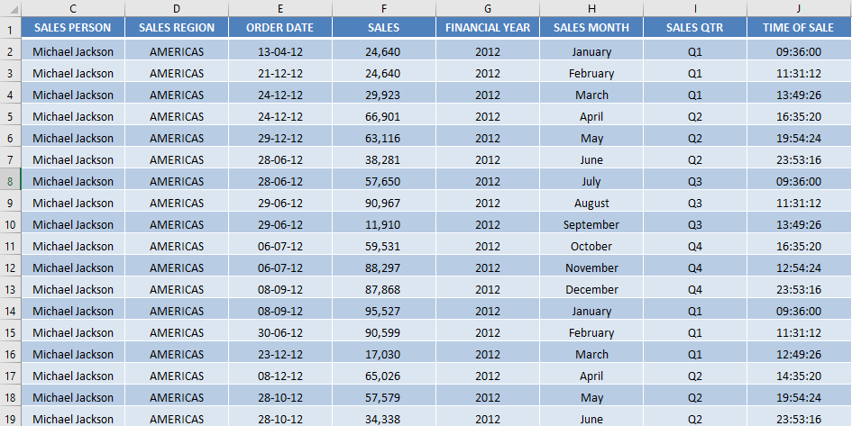
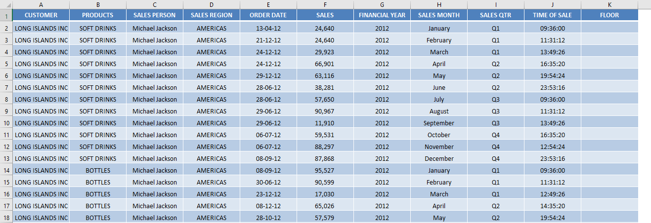
In the example below, you have Sales data and you want to get the Sales Grouped by Time.

STEP 1: Insert a new Pivot table by clicking on your data and going to Insert > Pivot Table > New Worksheet or Existing Worksheet

 

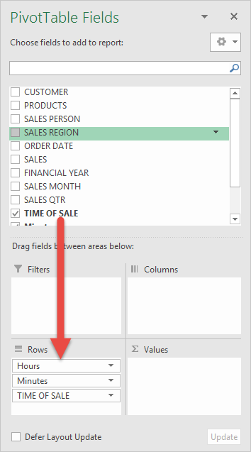
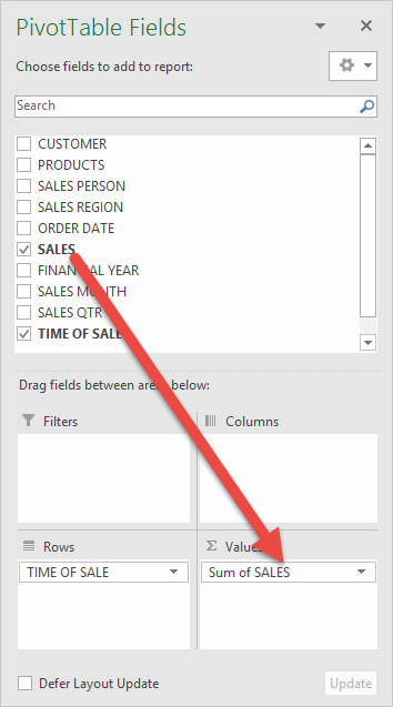
STEP 2: In the ROWS section put in the Time of Sale field.

Notice Excel will automatically Group the Time of Sale field in Excel 2016 (a new feature):

 

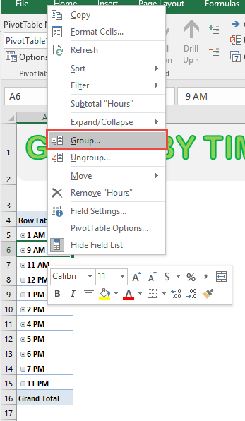
STEP 3: Right-click on any Row item in your Pivot Table and select Group

 

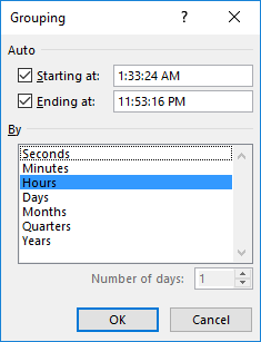
STEP 4: It was able to determine our time range (minimum time and maximum time).

Make sure only Hours is selected (blue highlight).

To create Excel Pivot Table group time by hour,  Click OK.

 

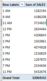
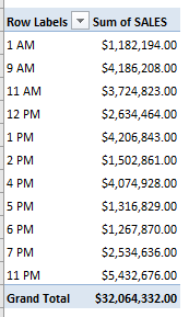
STEP 5: In the VALUES area put in the Sales field. This will get the total of the Sales for each hourly range you have defined:

Now we have our Excel Pivot Table group time by hour, notice that we can improve the formatting:

 

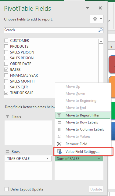
STEP 6: Click the Sum of SALES and select Value Field Settings

 

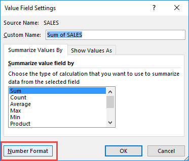
STEP 7: Select Number Format

 

STEP 8: Select Currency. Click OK.

You now have your total sales for each hourly period!

Extra Tip: You can Right Click on any Sales value in the Pivot Table and select Sort > Largest to Smallest.  This will show you the part of the day that has the most sales at the top!

The steps mentioned above can be used to Excel Pivot Table group time by hour.

 

Group by Custom Time Interval

There might be a time when you want to review the data based on a specific time block instead of a standard 1-hour interval. Like, you want the data to Excel Pivot Table group by 15 minutes or 2 hours or any other custom time interval.

You can easily do that using Excel’s FLOOR function.

Before we learn how to Excel Pivot Table group by 15 minutes, let’s first understand the FLOOR function and its use!
FLOOR Function in Excel can be used to round a number down to the nearest multiple of significance.

The Syntax of the FLOOR function is :

=FLOOR (number, significance)

where

• number – The numeric value you want to round
• significance – The multiple to which you want to round.

Luckily, Excel treats date and time as numbers. The integer portion of the number represents the day and the decimal portion represents the time.

The FLOOR function also accepts an argument in “hh: mm” format and it easily converts them to decimal values. For example, Excel converts 00:15 into 0.0104166666666667, which is the decimal value of 15 minutes, and rounds using that value.

 

Now, let’s take the same example and create an Excel Pivot Table group by 15 minutes.

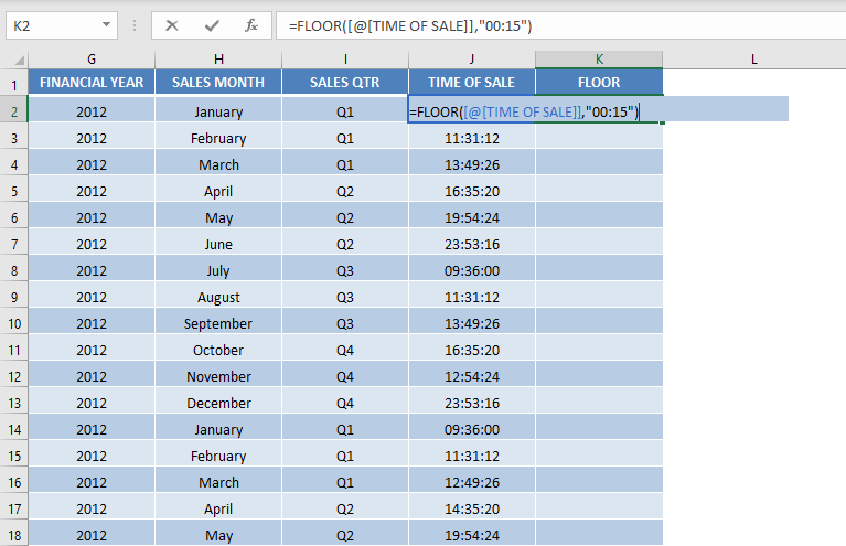
STEP 1: Insert a new column named FLOOR.

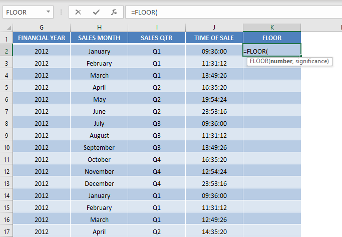
STEP 2: Insert the function FLOOR.

=FLOOR (

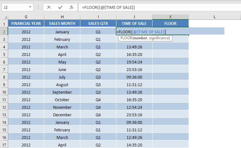
STEP 3: Insert the first argument – Time of Sales.

=FLOOR ([@TIME OF SALES]

STEP 4: Insert the second argument – significance. Here, it is 15 minutes ie 00:15.

=FLOOR ([@TIME OF SALES],”00:15″)

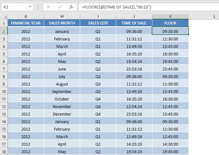
STEP 5: Copy-paste the formula down.

As you can the FLOOR function has rounded the time of sales in intervals of 15 minutes.

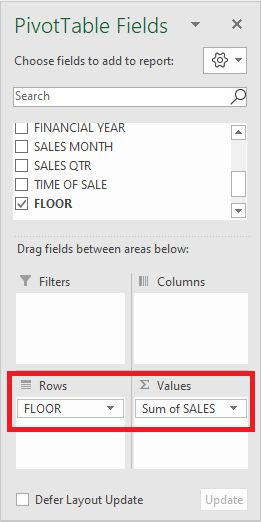
STEP 6: In the PivotTable Fields, drag and drop Time of Sales under Row column and Sales under Values column.

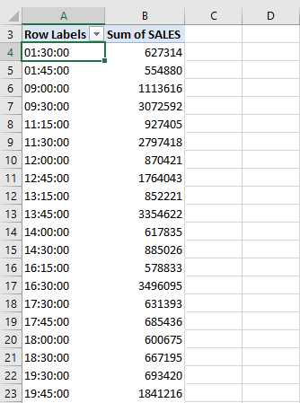
STEP 7: The columns will be displayed in the PivotTable.

This is how you can Excel Pivot Table group by 15 minutes!

 

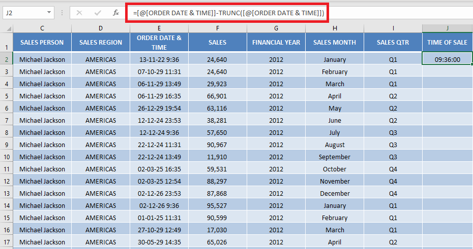
Pro-Tip: In case, you have data containing date and time together, you can easily extract time from that column and then perform the group feature.

 

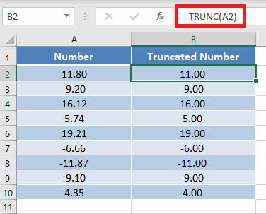
Before we move forward, let’s first understand how to remove decimal from a number in Excel. TRUNC function can be used to truncate a number by removing the decimal portion of a number.

It does not round off the number, it simply truncates the number.

For example, TRUNC(11.8) will return 11, and TRUNC(-9.2) will return -9.

 

Going back to the previous example! 

You can subtract the Date with time from the truncated date and will return only the decimal number. This will extract the time of sales.

This is how you can Pivot Table group by time range like every half hour “0:30” or every five minutes “0:05”.

Frequently Asked Questions

How can I group time by hour in an Excel Pivot Table?
To group time by hour, right-click on a time value in the Pivot Table, select Group, and then choose Hours in the grouping options. Excel will automatically group the data into hourly intervals.

Is it possible to group time data into custom intervals, like 15 minutes or 2 hours?
Yes, you can group time data into custom intervals. Right-click on the time value in the Pivot Table, choose Group, and set the Starting At, Ending At, and By fields to define your desired time interval (e.g., 15 minutes or 2 hours).

What should I do if the Group option is grayed out in my Pivot Table?
If the Group option is grayed out, ensure that the column containing time data is properly formatted as a time or date type. If the data contains text or blank cells, grouping will not work. Correct the format and try again.

Can I ungroup time data after grouping it in a Pivot Table?
Yes, you can ungroup time data at any time. Simply right-click on the grouped field in the Pivot Table and select Ungroup. The data will revert to its original format.

Will the grouped time intervals update automatically if the data changes?
Yes, the grouped intervals will automatically update if you refresh the Pivot Table after making changes to the underlying data. This ensures the grouped results remain accurate and reflect the latest updates.

Conclusion

If you wish you group time by 1-hour interval, you can simply use the group function available in Pivot Table.

But if you want to add a custom time interval like Excel pivot table group by 15 minutes, you can use the floor function to round off the time to a custom interval.