Highlight All Excel Formula Cells

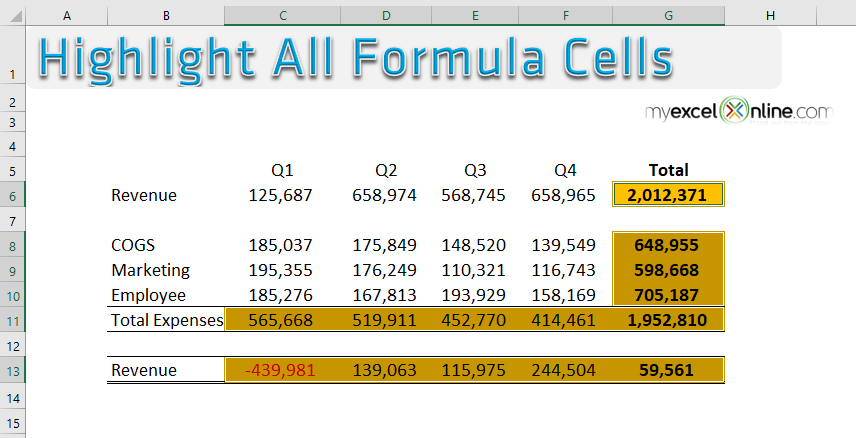
Whenever you are auditing an Excel worksheet and need to know where all the formulas are located, a great way is to highlight the formula cells in a distinctive color.  You will be surprised how easy it is to do this, especially when you need to review the formulas to find if there is an issue.

Key Takeaways:

• Quick Formula Identification: Highlighting formula cells allows you to easily identify where calculations are being performed, simplifying data auditing and troubleshooting.
• Built-In Excel Feature: You can quickly highlight all formula cells using the Go To Special feature, which eliminates the need for manual searching across the worksheet.
• Enhanced Data Transparency: Highlighted formula cells stand out from static values, making it easier to differentiate between calculated and manually entered data in large spreadsheets.
• Customizable Formatting: Once selected, you can apply custom formatting, such as bold text or colored fills, to formula cells, improving visual clarity and accessibility.
• Improves Collaboration: Highlighted formulas help team members or collaborators quickly understand which cells depend on calculations, reducing errors during data editing or review.

How to Highlight All Excel Formula Cells

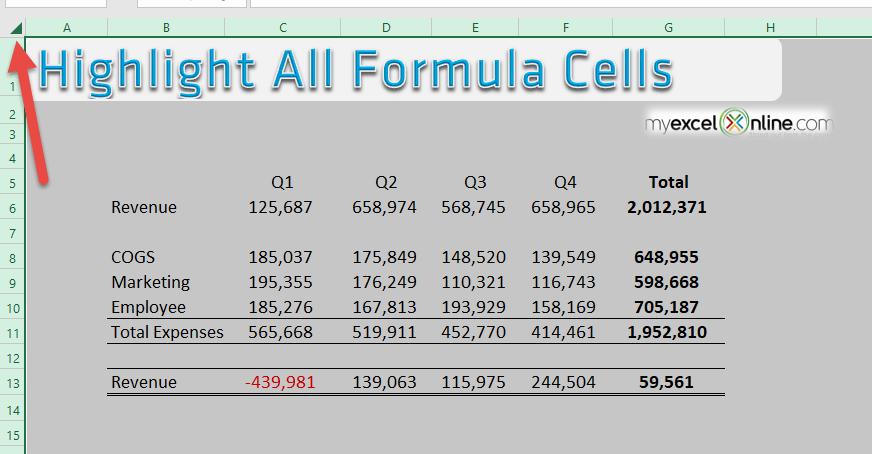
STEP 1: Select all the cells in your Excel worksheet by clicking on the top left hand corner of your worksheet.

 

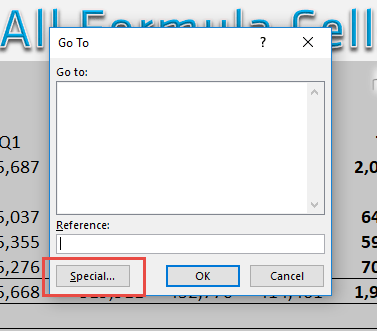
STEP 2: Press the CTRL+G shortcut which will open up the Go To dialogue box and select the Special button.

 

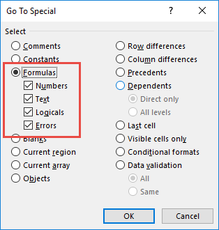
STEP 3: Select the Formula radio button and press OK.

 

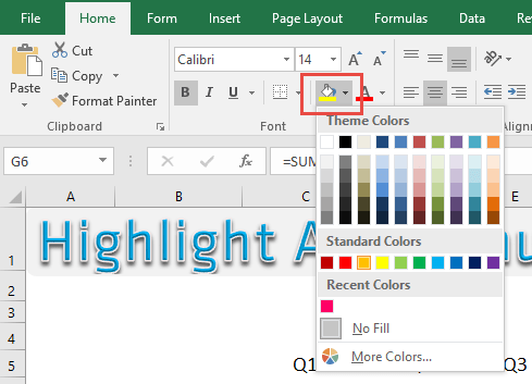
STEP 4: This will highlight all the formulas in your Excel worksheet and you can use the Fill Color to color in the formula cells.

And now all your cells containing formulas are now highlighted!

 

Saving Time with Excel Shortcuts and Quick Analysis

Master Key Shortcuts for Conditional Formatting

Embrace the power of Excel’s keyboard shortcuts to navigate Conditional Formatting like a pro. They help you apply, manage, and clear formatting rules at warp speed, making your workflow smoother and more intuitive.

For instant access to Conditional Formatting options, press Alt + H + L. This hotkey combo instantly summons the menu, allowing you to swiftly implement new rules or adjust existing ones. To craft a new rule with ease, Alt + H + L + N is your go-to sequence, leading you directly into the rule creation dialogue.

When the aim is to breeze through the editing of rules, remember Alt + O + D. This command opens the Conditional Formatting Rules Manager, laying out all your rules neatly for review or alteration. Should you need to remove a rule from the selected cells, Alt + H + L + D offers a one-shot solution to declutter your cell formatting.

Speaking of de-cluttering, if you’re looking to wipe the slate clean and remove all Conditional Formatting from a selection, Alt + H + L + C will do the trick, echoing the command for a fresh start.

Be mindful, though, as shortcuts can differ based on your Excel version or operating system. Make sure to review the list of shortcuts pertinent to your specific setup for the smoothest sailing.

Leveraging Quick Analysis for Instant Results

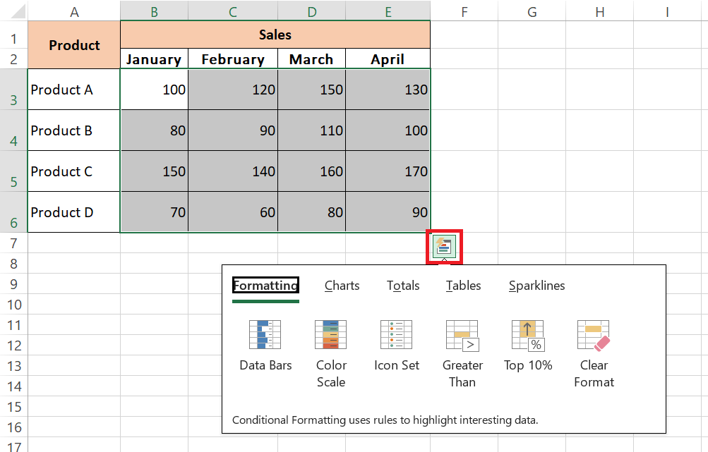
Discover the joys of the Quick Analysis tool in Excel, a real game-changer for those who seek to add visual flair and analytical depth to their data at lightning speed. Simply select a range of cells containing data and watch for the magic Quick Analysis button that appears like a trusty genie, ready to grant your data-related wishes.

Give the Quick Analysis button a click, or for those who love saving time, press Ctrl + Q to unveil a treasure trove of options including formatting, charts, totals, tables, and sparklines. Want to highlight your top performers or draw attention to the outliers? Conditional Formatting choices unveil themselves, letting you do just that with options like Color Scales, Icon Sets, and Data Bars.

And it doesn’t stop at visual treats—Quick Analysis is also your shortcut to deriving insights swiftly. Want to insert a sum or average? The Totals tab lays out functions in a neat row for you to select and apply without a second thought. If you’re in the mood to transform your data into a visually compelling story, charts and sparklines emerge at your service with just a click or two.

Excel’s Quick Analysis tool is like having a data assistant by your side, offering up suggestions and swiftly implementing your decisions, allowing you to move from data to insights with elegance and speed.

Frequently Asked Questions

How can I quickly highlight all formula cells in an Excel worksheet?

To highlight formula cells, go to the Home tab, click Find & Select in the Editing group, and choose Go To Special. In the dialog box, select Formulas and click OK. All formula cells will be selected, and you can apply formatting, such as a fill color, to highlight them.

Can I use conditional formatting to automatically highlight formula cells?

No, conditional formatting cannot directly detect formulas. However, you can use the Go To Special feature to manually identify and format formula cells.

Does highlighting formula cells affect their functionality?

No, highlighting formula cells only changes their appearance (e.g., color or font style) and does not alter the functionality or results of the formulas.

Can I highlight formula cells across multiple sheets at once?

The Go To Special feature works only on one worksheet at a time. To highlight formula cells on multiple sheets, you need to repeat the process for each sheet or use a VBA macro for automation.

Why should I highlight formula cells in my worksheet?

Highlighting formula cells makes it easier to differentiate between calculated values and static data, especially in large datasets. It simplifies data auditing, reduces errors, and helps collaborators quickly understand the structure of your worksheet.