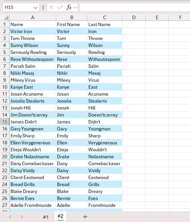
Highlight alternate rows in Microsoft Excel will significantly boost the readability and visual appeal of data tables. By introducing a clear distinction between rows, this formatting technique helps to reduce eye strain and facilitate quicker data comprehension. It plays a key role in highlighting patterns, trends, and enhancing the professional appearance of reports.
Key Takeaways
- Visual Clarity: Alternate row coloring in Excel enhances visual distinction, making it easier to follow complex data sets.
- Easy Methods: Utilize Excel Table Styles for quick application or Conditional Formatting for more customized control.
- Excel Table Feature: Convert data into a table for immediate formatting improvements and customizable options.
- Conditional Formatting: Offers precision in data visualization, allowing for tailored row highlighting based on specific conditions.
Table of Contents
Introduction to Coloring Excel Rows
The Visual Benefits of Highlighting Alternate Rows
Highlighting alternate rows in Excel significantly enhances the visual appeal and readability of data tables, by providing a clear distinction between each row. This formatting technique helps reduce eye strain and allows users to follow along more easily, facilitating quick comprehension of complex datasets.
It also aids in identifying patterns and trends at a glance, which is crucial for effective data analysis. Moreover, the professional appearance of color-coded tables improves the overall presentation of reports and documents.
Quick Overview of Methods for Applying Row Shading
Highlighting alternate rows in your Excel sheet not only enhances readability but also allows for quick data assessment at a glance. There are primarily two easy methods to achieve this:
- Excel Table Styles: Instantly apply alternating row colors by converting your data into a table and selecting from an array of predefined styles.
- Conditional Formatting: Gain more control and customize how you apply the color bands across your rows based on certain conditions or values.
Both methods are straightforward and can be applied with a few clicks, bringing a structured and polished look to your data. Let’s dive in and discover how you can utilize these techniques for efficient data visualization.
Step-by-Step Guide to Alternate Row Shading
Transform Your Data with Excel’s Built-in Table Feature
Unleash the full potential of your data visualization with Excel’s built-in Table feature. It’s not just about neat rows; it’s the foundation for managing and analyzing your data efficiently.
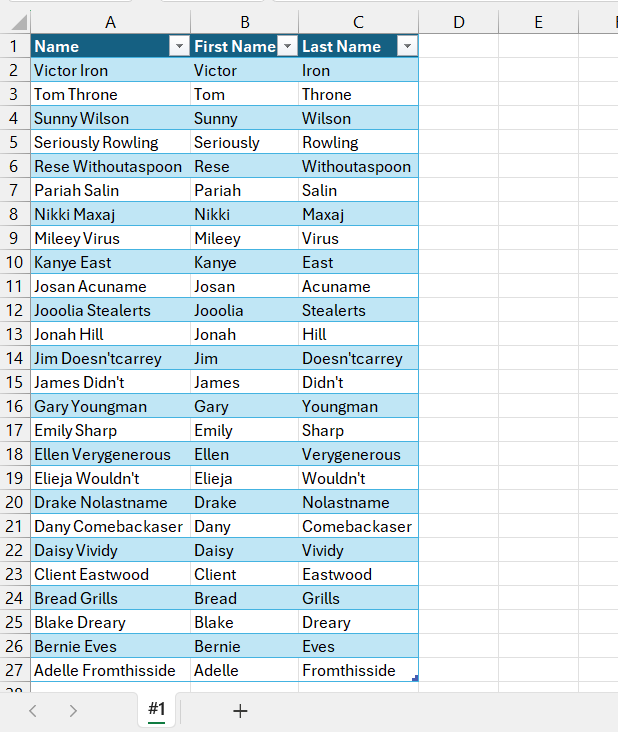
Simple Conversion: With just a few clicks, you can convert your data range into a structured table and see the transformation as Excel applies a clear format, replete with alternating row colors for immediate visual enhancement.
Customization at Fingertips: If the default styles don’t match what you’re looking for, no worries! Excel allows you to modify the shades, fonts, and borders to create a custom look that aligns with your preferences.
Step-by-Step:
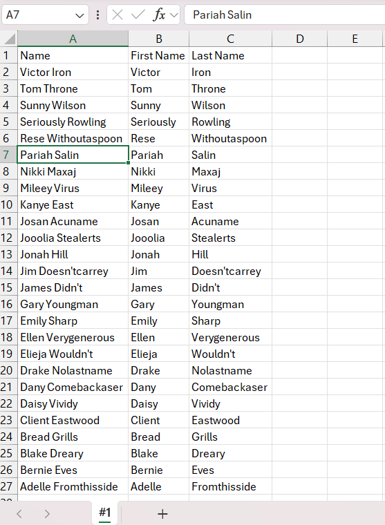
STEP 1: Click any cell within your data range.
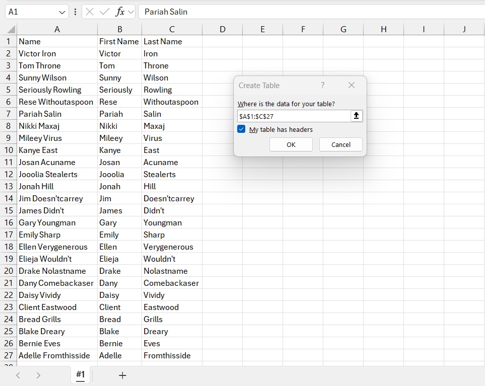
STEP 2: Navigate to Insert > Table or simply use the keyboard shortcut Ctrl + T.
STEP 3: In the dialog box, confirm if your data includes headers and click OK.
STEP 4: Witness as Excel wraps your data in a table with a distinct style, including banded rows.
After these quick steps, you’re all set with a neatly organized table that not only looks good but is also primed for further analysis and manipulation—talk about a smart upgrade!
Conditional Formatting: The Smart Way to Distinguish Data
Excel’s Conditional Formatting is like having a keen-eyed assistant that differentiates your data for you. It’s smart, attentive, and remarkably adaptable to your unique data requirements.
Pinpoint Precision: It goes beyond the basics to let you stipulate exactly how and when rows should be highlighted. You tell Excel the when, and it takes care of the how.
Deeper Data Connection: It’s not just about alternating colors for aesthetics—the patterns you create can reflect the underlying nature of the data itself. Whether it’s grouping similar items or flagging outliers, conditional formatting adds depth to your data’s story.
Step-by-Step:
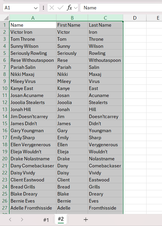
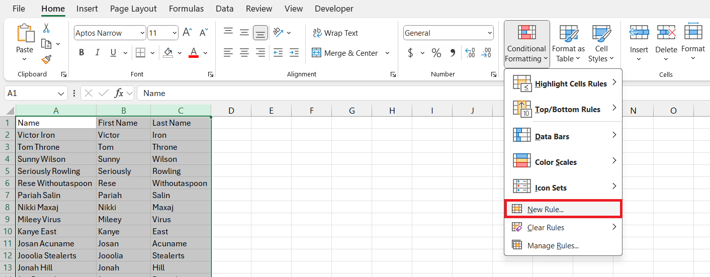
STEP 1: Click on the column header to select the rows you want to format.
STEP 2: Go to Home > Conditional Formatting > New Rule.
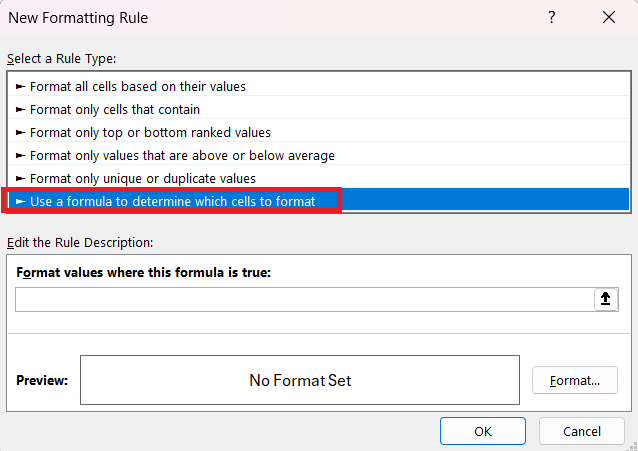
STEP 3: Choose the ‘Use a formula to determine which cells to format’ option.
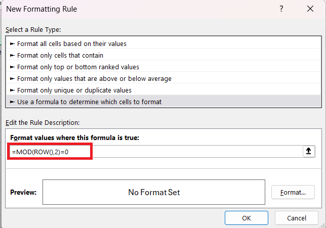
STEP 4: Enter the formula to identify alternate rows (e.g., =MOD(ROW(),2)=0 for even rows).
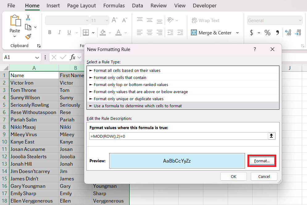
STEP 5: Select the Format button, decide on your fill color, and click OK to apply.
Alternate rows will be highlighted –
The formula =MOD(ROW(),2)=0 is used in a spreadsheet to determine if a row is even-numbered. Here’s a breakdown of how it works:
- ROW(): This function returns the row number of the cell where the formula is located. For example, if the formula is in any cell in row 5, ROW() returns 5.
- MOD(number, divisor): The MOD function returns the remainder after dividing the number by the divisor. In the formula =MOD(ROW(),2), it calculates the remainder of dividing the current row number by 2.
- =MOD(ROW(),2)=0: This part of the formula checks if the remainder of the division is zero. If the remainder is zero, it means that the row number is divisible by 2, indicating that it is an even row. The formula thus evaluates to TRUE for even rows and FALSE for odd rows.
This formula is particularly useful in conditional formatting, where you might want to apply a specific formatting style to even rows to improve readability by creating a striped pattern in a list or table.
As you follow these steps, marvel at how rows light up in response to your commands, drawing attention precisely where it’s needed. This smart way to distinguish data isn’t just about appearance; it’s about adding layers of meaning to your spreadsheets.
Maximizing Efficiency with Excel Productivity Hacks
Keyboard Shortcuts to Speed Up Formatting Tasks
Keyboard shortcuts are like hidden pathways in a labyrinth—know them, and you’ll navigate through your tasks with enviable ease and speed. When it comes to formatting in Excel, knowing the right keys to press can cut down on clicks and menus, saving you precious time.
Shading Shortcuts: For starters, the simple yet mighty Alt + H + H shortcut opens the floodgates to Excel’s color palette, letting you swiftly apply your desired hue to the selected cells.
Best Keyboard Shortcuts for Formatting:
- Alt + H, L: This opens the Conditional Formatting menu right from your keyboard.
- Ctrl + T: Instantly convert your data range into a table, making alternating color formatting automatic.
- Alt + E, S, T: Copy a cell’s format and paste it elsewhere with this sequence.
- Ctrl + 1: Brings up the Format Cells dialog box for all-encompassing cell customization.
- Alt + O, R, A: Auto-adjust row heights to fit the content perfectly.
Incorporating these shortcuts into your workflow will not only impress your peers but also give you more time to focus on what your data is telling you rather than on how you’re presenting it.
FAQs about Highlighting Rows in Excel
How Do I Apply Alternating Colors to Rows Without Using a Table?
To apply alternating colors to rows in Excel without using a table, leverage Conditional Formatting:
- Select the range of rows you wish to format.
- Go to the Home tab and click Conditional Formatting.
- Choose “New Rule” and select “Use a formula to determine which cells to format”
- Enter the formula
=MOD(ROW(), 2) = 0to select even rows. - Click on “Format,” choose your color under the Fill tab, and hit OK.
This method gives you the flexibility to choose any color combination for your alternating rows, independent of the table feature.
Is it possible to alternate rows using more than two colors?
Absolutely! In Excel, you can use conditional formatting to apply more than two colors across alternating rows. Simply create multiple rules with different formulas—like =MOD(ROW(),3)=1—and assign various colors. This allows you to introduce a multi-colored pattern for better visualization or categorization.
What Should I Do if Conditional Formatting Isn’t Working?
If Excel’s conditional formatting isn’t working, first check that your rules are set correctly. Confirm the range applies to your intended cells and that there are no conflicting rules. Also, double-check any formulas for accuracy, and ensure that they’re not formatted as text. If problems persist, clearing all rules and reapplying them can often rectify issues.
Is It Possible To Highlight Alternate Rows in Large Datasets Efficiently?
Yes, it’s possible to efficiently highlight alternate rows in large datasets. Utilize Conditional Formatting with an appropriate formula, like =ISEVEN(ROW()), to handle large volumes of data without manually coloring each row. This method ensures quick, automatic, and error-free shading across your dataset.
How do you select every alternate row in Excel?
To highlight the second row in Excel, click on the header of row 2 to select the entire row. Then, go to the “Home” tab on the ribbon, and click on the “Fill Color” icon (it looks like a paint bucket) to choose your desired highlight color. This will apply the selected color to the entire second row.
John Michaloudis is a former accountant and finance analyst at General Electric, a Microsoft MVP since 2020, an Amazon #1 bestselling author of 4 Microsoft Excel books and teacher of Microsoft Excel & Office over at his flagship MyExcelOnline Academy Online Course.

