Highlight Alternate Rows in Selection Using Macros In Excel

When it comes to highlighting alternate rows in your data, it’s a cumbersome process! One way is to use the table formatting option in Excel, but you can also use Excel Macros to highlight alternate rows for you!

And you have full control on how it will look like!

Make sure your Excel has the Developer Tab enabled following this tutorial.

I explain how you can do this below step by step!

What does it do?

Highlights alternate rows in your selection

Copy Source Code:

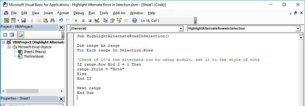
Sub HighlightAlternateRowsInSelection()

Dim range As Range
For Each range In Selection.Rows

'Check if it's the alternate row by using modulo, set it to the style of note
If range.Row Mod 2 = 1 Then
range.Style = "Note"
Else
End If

Next range
End Sub

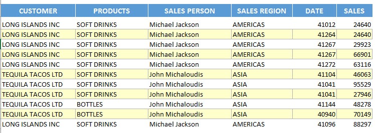
Final Result: 

Exercise Workbook:

---

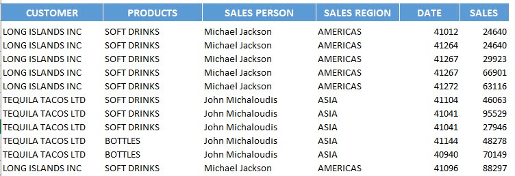
Here is our initial set of data:

STEP 1: Go to Developer > Code > Visual Basic

 

STEP 2: Paste in your code and Select Save. Close the window afterwards.

 

STEP 3: Let us test it out!

Open the sheet containing the data. Go to Developer > Code > Macros

 

Make sure your data and macro are selected. Click Run.

With just one click, the alternate rows of your selection are now highlighted!

 How to Highlight Alternate Rows in Selection Using Macros In Excel