5 Epic Ways to Highlight Duplicates in Excel

In Excel, you are usually working with a large dataset, and encountering a duplicate value is really common. It may lead to incorrect formulas or calculations making the data inconsistent or inaccurate. You can easily spot and highlight duplicates in Excel using a really versatile feature – Conditionally Formatting. If you are not unfamiliar with this feature, it would be a good idea to go through it before we proceed.

Download the Excel Workbook below to follow along and understand how to highlight duplicates in Excel –

download excel workbookHighlight-Duplicates-in-Excel.xlsx

Key Takeaways:

• Conditional Formatting is a powerful tool in Excel for identifying and highlighting duplicate values. To utilize this feature, one simply needs to select the range with potential duplicates, and then apply Conditional Formatting from the Home Ribbon. This will visually distinguish duplicate entries by applying a chosen color to the cell or text, making it easier to manage and analyze data.
• For those who prefer keyboard shortcuts for efficiency, Excel offers a quick method to highlight duplicates. By sequentially pressing ALT, followed by H, L, H, and D, users can swiftly apply the duplicate highlighting rule to a selected range of cells. This shortcut streamlines the process, saving time and effort during data analysis tasks where duplicate identification is critical.
• Handling large datasets often requires continuous monitoring for duplicates as data grows. To maintain consistent oversight of duplicates, simply apply the Conditional Formatting rule to entire columns where new data will be added. This ensures that any future duplicates are automatically highlighted, sustaining data integrity and simplifying the task of keeping your Excel spreadsheets clean and accurate as your dataset evolves.

Highlight Duplicates using Conditional Formatting

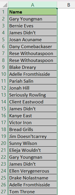
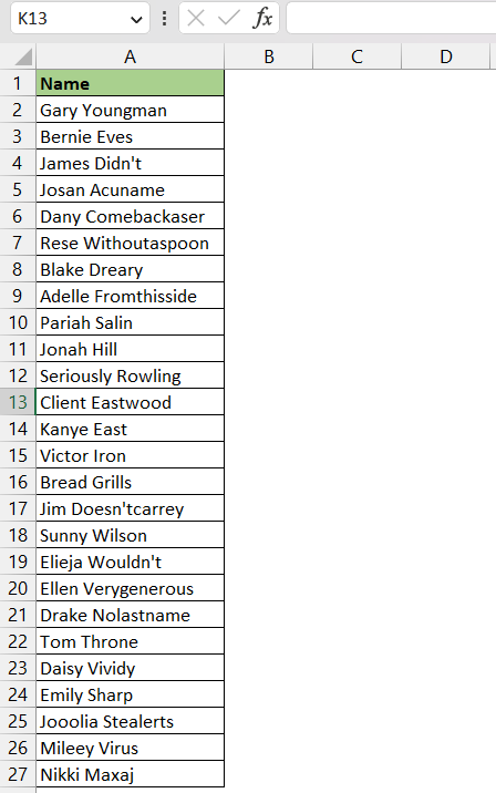
There is an in-built feature in conditional formatting that can be used to highlight duplicates. In this example, you have a list of employee names in Column A and you want to highlight the duplicate ones in red. Follow the steps below to apply it –

STEP 1: Select the range that contains duplicate values.

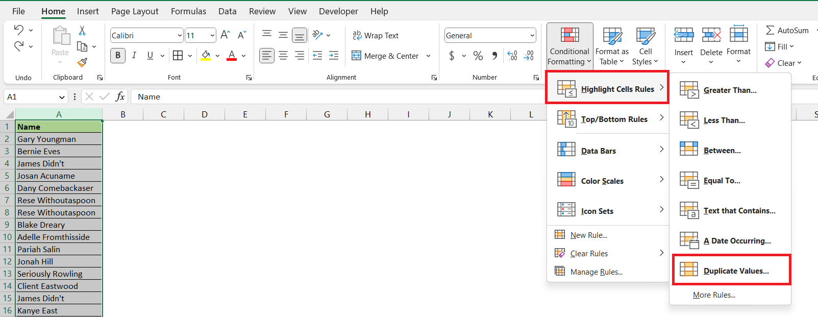
STEP 2: Go to the Home Tab > Click on Conditional Formatting in the Styles group.

STEP 3: Select Highlight Cells Rules > Duplicate Values.

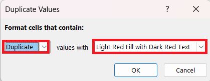
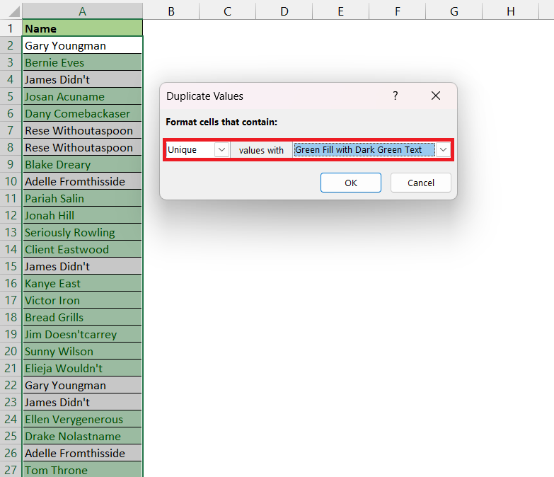
STEP 4: In the Duplicate Values dialog box, select Duplicate and then the formatting that you want to apply. In this example, let’s select Light Red Fill with Dark Red Text.

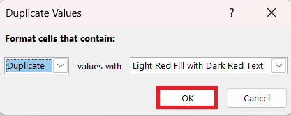
STEP 5: Click OK.

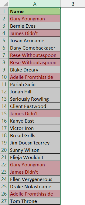
You can see that all the duplicate values in the range will be highlighted based on the formatting that you have selected.

Pro Tip – In the dropdown, you can select Unique and all the unique values will be highlighted in the range.

 

Highlight Duplicates expect 1st Occurence

In the previous example, what if you want to highlight all duplicates except the first occurrence? Excel has a way around that – you need to use a combination of the COUNTIF function and conditional formatting.

Follow the steps below –

STEP 1: Select the range that contains duplicate values.

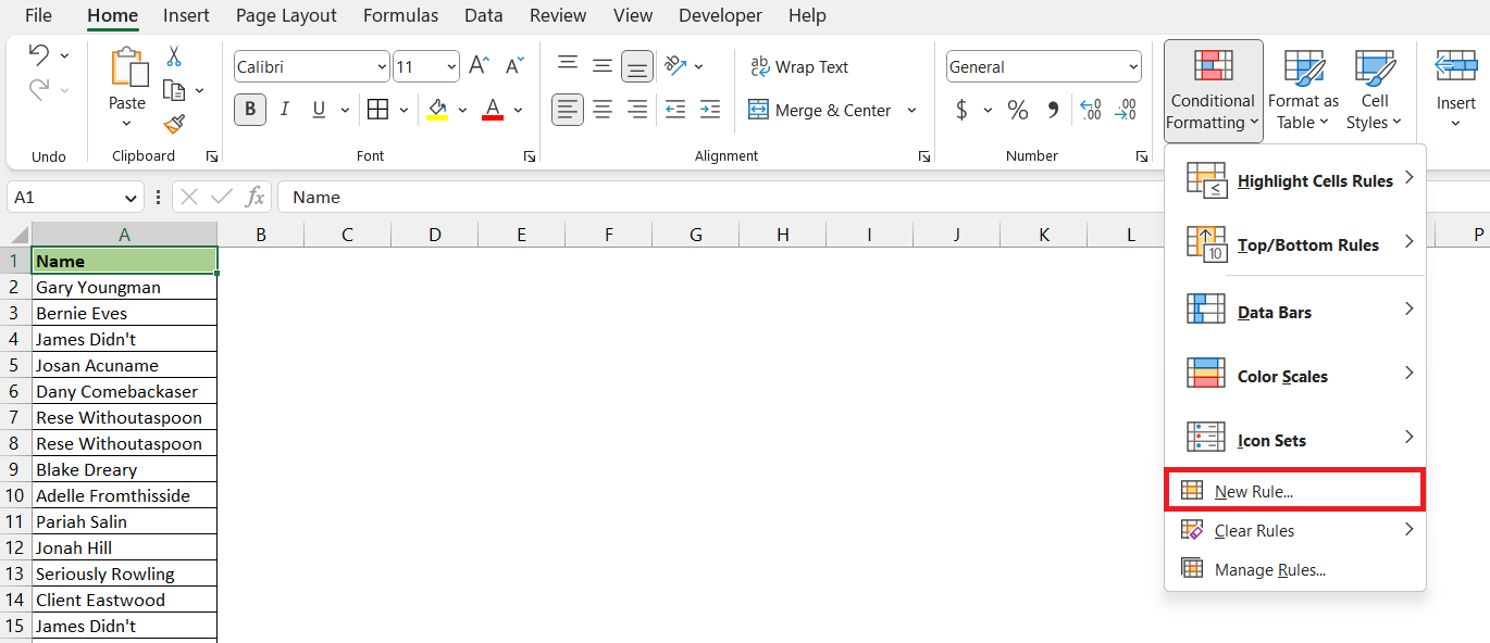
STEP 2: Go to the Home Tab > Click on Conditional Formatting in the Styles group.

STEP 3: Go to New Rule.

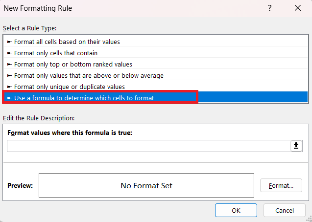
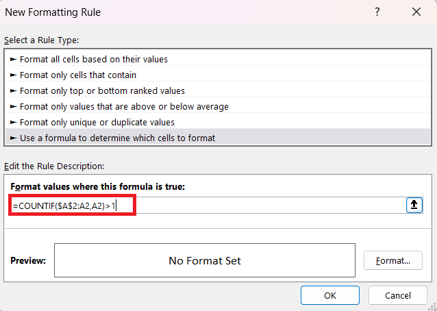
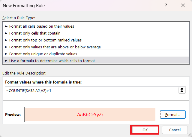
STEP 4: In the New Formatting Rule dialog box, select Use a formula to determine which cells to format.

STEP 5: Enter the following formula in the Edit Rule Description section –

=COUNTIF($A$2:A2,A2)>1

Here, we are using a mixed reference range ($A$2:A2) -where the first cell in the reference is locked ($A$2) and the second range is left relative (A2). As you copy the formula down, the range will keep accommodating a new row. So, the COUNTIF formula will check values from the first location ($A$2) till the current location (say, A5) and will avoid the values below (from A6 to A32).

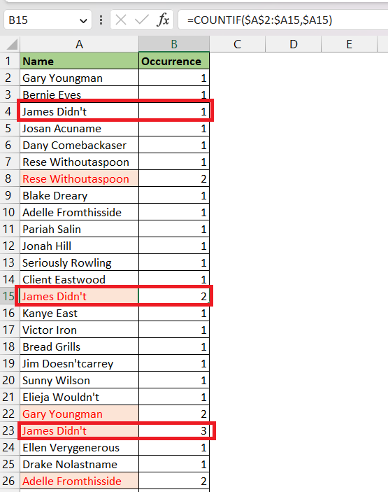
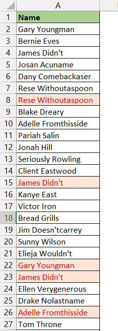
For example, when COUNTIF is running the formula in cell A15, it will count the occurrence of “James Didn’t” from A2 to A15 and will display the result i.e. 2. It will not take into consideration the names mentioned in the range A16 to A32.

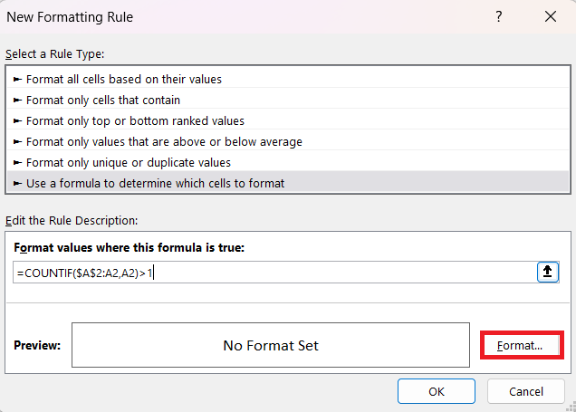
STEP 6: Click on the Format button.

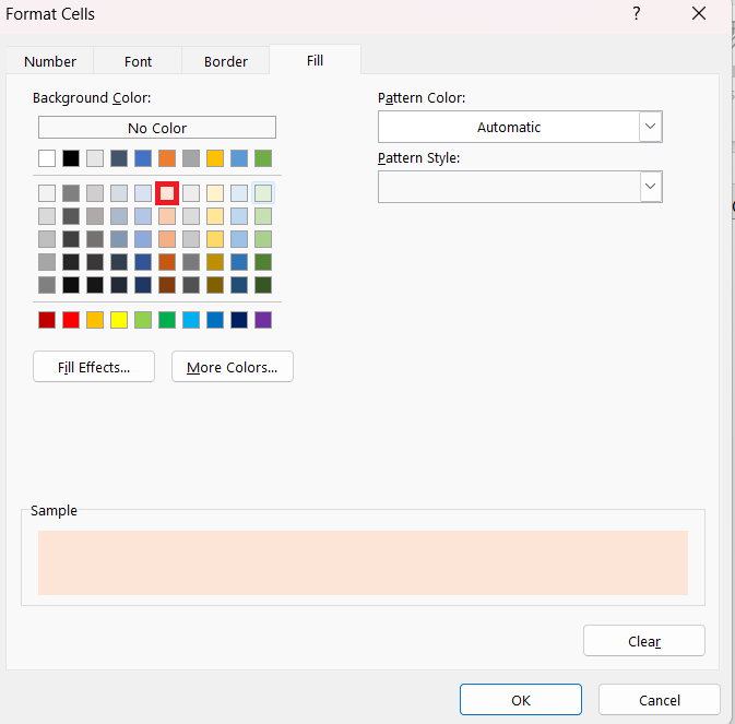
STEP 7: Go to the Fill tab and select a light red color.

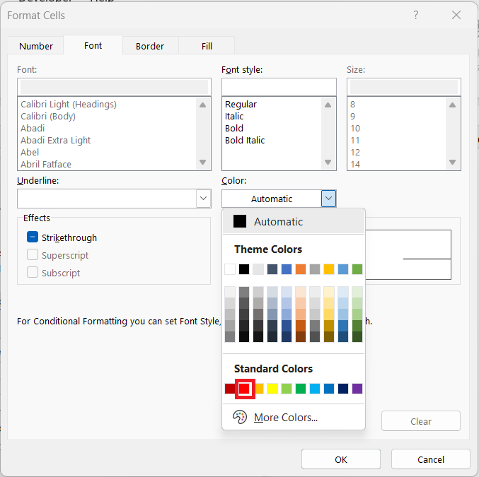
STEP 8: Go to the Font tab and select a red color.

STEP 8: Double-check the formatting for duplicates in the Preview section and press OK.

All the duplicates except the first occurrence has been highlighted in red font and light red fill.

 

Highlight Duplicate Rows

Until now, we analyzed and highlighted duplicates based on values entered in a cell. The in-built feature of conditional formatting looks for value cell by cell only. Now, we want to look at the entire row’s content and then check for duplicates.

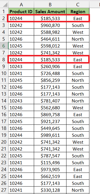
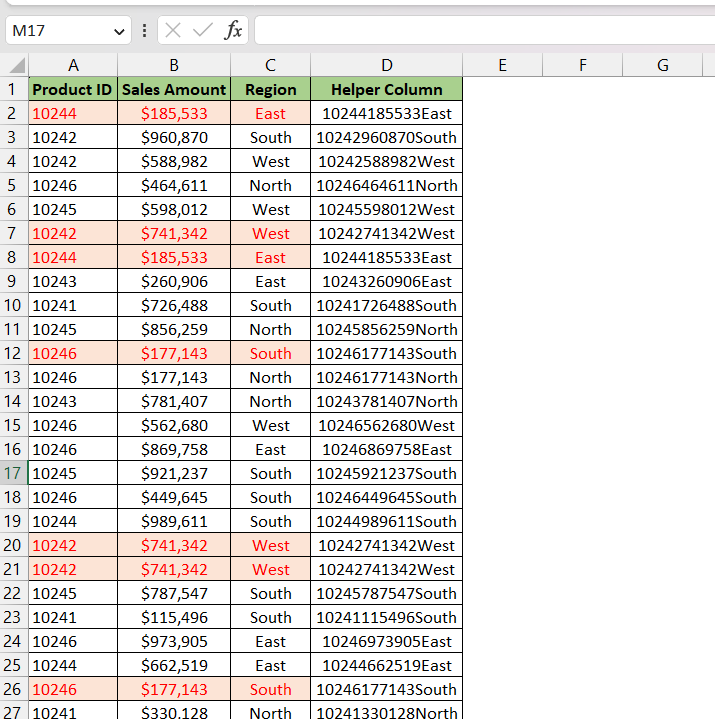
In this example, we want to highlight a row only when values in all three columns are the same for any 2 rows.

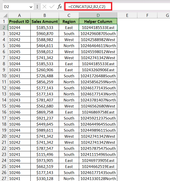
We will be using the CONCAT function to create a helper column that will help us in highlighting duplicate rows. Follow the steps below to highlight duplicate rows –

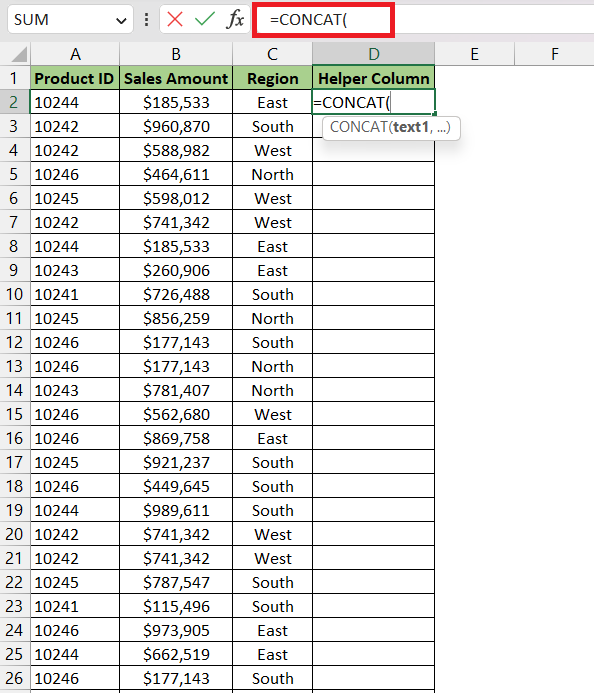
STEP 1: Go to cell D2 and enter the CONCAT function.

STEP 2: Select all three cells that you want to combine. and copy the formula down.

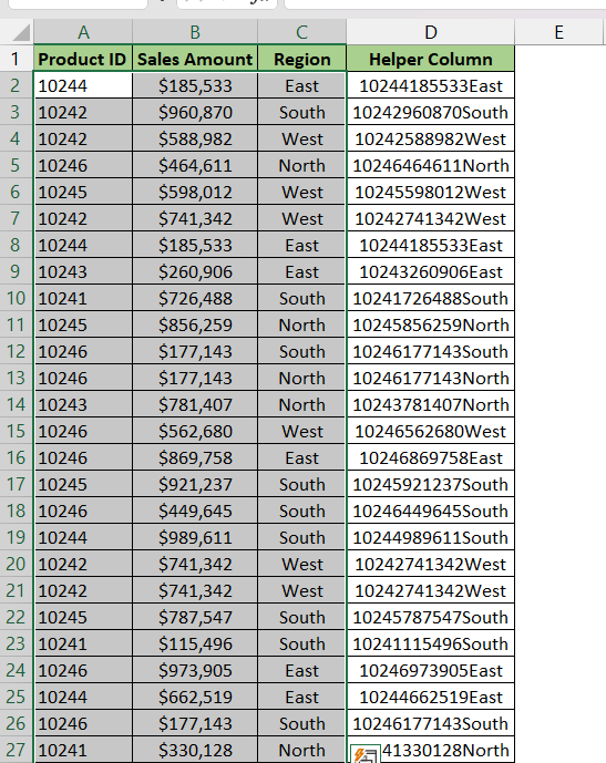
We will be using range A2:C32 to highlight duplicates and range D2:D32 to check for duplicates.

STEP 3: Select the range where you want to highlight duplicates i.e. A2:C32.

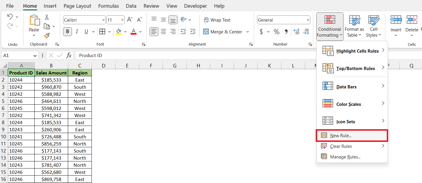
STEP 4: Go to Home > Conditional Formatting > New Rule.

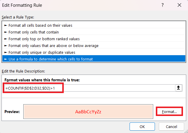
STEP 5: In the New Formatting Rule dialog box, enter the following formula –

=COUNTIF($D$2:D32,$D2)>1

Now, select the formatting that you want and press OK.

All the duplicate rows have been highlighted.

 

Remove Duplicates

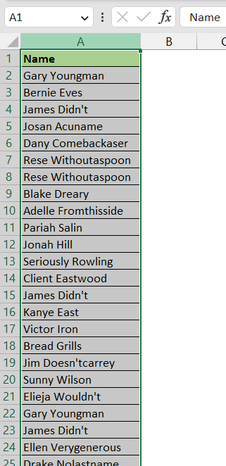
Instead of highlighting duplicates in the list, you may sometimes want to simply remove those duplicates from the list. Let’s see how it can be done:

STEP 1: Select the range containing duplicate values.

STEP 2: Go to Data > Remove Duplicates.

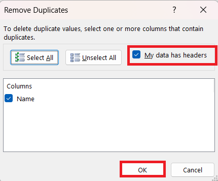
STEP 3: In the dialog box, check My data has headers and click OK.

STEP 4: Excel sends an alert stating the number of duplicates that have been removed and the remaining number of unique values. Click OK.

All the duplicates have been removed and the list now contains only unique values.

 

Put Unique Values in Another Column

What if we don’t want to highlight duplicates or remove them, we simply want out the unique values in another column?

Excel has a function for this as well- UNIQUE. If you are unable to find this formula, you may be using an older version of Excel. Click here to download Excel 365 and enjoy the benefits of using this amazing function.

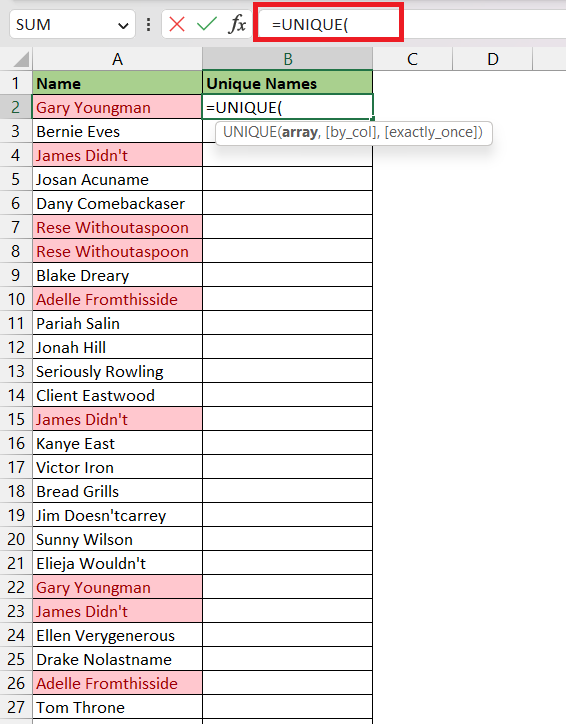
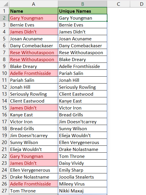
In this example, we have a list of names in column A that contains duplicates. We want to get a list of unique names in column B without making any change in column A. Let’s see how it can be done.

STEP 1: Enter the UNIQUE function in cell B2.

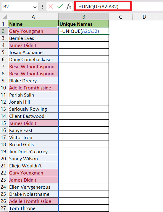
STEP 2: Select the data from which you want to remove duplicates.

All the unique names will be listed in column B.

Important Considerations When Dealing with Duplicates

Potential Pitfalls to Avoid

When tackling duplicates in Excel, you want to tread carefully. The main trap to avoid is the accidental deletion or mislabeling of crucial data. Sometimes, what appears to be a duplicate could have subtle differences that are important. Therefore, cross check your entries meticulously before doing any clean-up. Also, ensure your actions are reversible—always have a backup of your original data!

Ensuring Data Integrity Post-Highlighting

After highlighting duplicates, it’s paramount to preserve the accuracy and consistency of your dataset. To ensure data integrity, audit your highlighted entries to confirm they’re true duplicates. Review relationships between data points to avoid breaking links with other essential data. Also, consider documenting the steps taken during the cleaning process, which allows for tracing back and understanding the rationale behind each action if questions arise later on.

Keyboard Shortcuts for Quick Highlighting

Excel shortcuts are your best friends when it comes to improving your efficiency. To quickly highlight duplicate values, you don’t have to go through numerous menu steps; just use the combination ALT → H → L → H → D. Remember, each key is pressed separately, unlocking a tier of commands in sequence, not all at once. Shortcuts like these can turn a tedious task into a swift action, freeing up your time to focus on more complex data analysis.

Taking Action: What to Do After Highlighting Duplicates

Removing Duplicates with Confidence

Removing duplicates confidently entails verifying your selections before confirming deletions. Utilize the ‘Remove Duplicates’ feature under the ‘Data’ tab in Excel, but first, ensure you’ve backed up your original dataset. Select the columns you want to check for duplicates carefully. Remember, any deselected columns will be ignored even if they contain duplicate content. Confirm the action and Excel will inform you of how many duplicates were removed and how many unique values remain.

Analyzing Data Post-Duplicate Management

Once duplicates are identified and addressed, it’s time to dive back into your analysis with a renewed perspective. With duplicates out of the way, your analysis won’t be skewed by redundant data. Look for patterns, trends, and anomalies with fresh eyes, and use pivot tables or charts to visualize the refined information. This will lead to more accurate insights and informed decision making, allowing for a clearer interpretation of your data’s story.

Frequently Asked Questions

How do I highlight duplicates in Excel using only formulae?

To highlight duplicates in Excel using formulae, use Conditional Formatting with a custom formula. For example, to highlight duplicates in the range B4:G11, use the formula =COUNTIF($B$4:$G$11, B4)>1. This will flag any cell in your selection that appears more than once. Remember to apply the formula relative to the “active cell” in your selection.

Can I highlight duplicates across multiple worksheets or workbooks?

Yes, you can highlight duplicates across multiple sheets or even different workbooks, but it requires more advanced Excel functions. You would use formulas that reference different sheets or workbooks. For instance, using 3D referencing or a VLOOKUP function could help you identify and then conditionally format duplicates across sheets or workbooks.

Is it possible to keep the first occurrence unhighlighted when identifying duplicates?

Absolutely, you can keep the first occurrence of a value unhighlighted when identifying duplicates in Excel. To do this, set up Conditional Formatting with a formula that only highlights the second and subsequent instances. A formula like =COUNTIF($A$2:A2, A2)>1 will do the trick when applied to a range, as it counts how many times the value has appeared up to the current row.

What are some common mistakes to avoid when highlighting duplicates in Excel?

When highlighting duplicates in Excel, avoid common mistakes like not specifying the correct range, resulting in incomplete checks. Remember that highlighting is case-sensitive; thus, confirm whether this impacts your data. Also, beware of accidental overwrites if using formulas to flag duplicates. Ensure you’re considering the entire dataset if it spans multiple columns, and always keep a backup before making changes to your data.

In this article, we have learned how to highlight duplicate values and rows, how to highlight all except 1st occurrence of duplicates, remove duplicates and get unique values in a new column.