Conditional Formatting Tips: Highlight Rows that starts with D in Excel

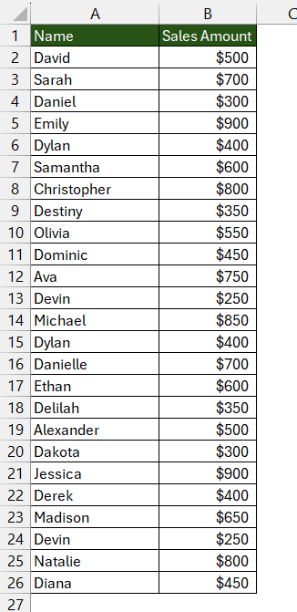
Microsoft Excel offers a powerful feature known as Conditional Formatting, which allows users to automatically apply specific formatting to rows based on the contents of cells. This tutorial will guide you through the steps to effortlessly highlight rows that starts with d in Excel. Whether you are analyzing a financial report or tracking project milestones, mastering this function can significantly improve your efficiency in Excel.

Key Takeaways

• Excel’s conditional formatting emphasizes key data, aiding the intuitive and efficient analysis of large datasets.
• Highlighted rows in Excel draw attention to important information, aiding in categorization, pattern recognition, and overall data comprehension.
• Before formatting, organize and backup your data to streamline the process and mitigate potential errors.
• Highlighting rows that start with D in Excel involves a straightforward process of creating a custom formula, enhancing data clarity and analysis.

Download the spreadsheet and follow the tutorial on How to highlight rows that starts with D in Excel – Download excel workbookHighlight-row-starts-with-d.xlsx

 

Introduction to Conditional Formatting

Conditional formatting enables the application of specific formatting styles to cells, contingent upon meeting predefined criteria. This helps you visually emphasize important data points within large datasets, making it easier to analyze and comprehend information at a glance.

Significance of Highlighting Rows for Data Analysis

Highlighting rows in Excel is a game-changer for data analysis. When you’re working with vast sheets, it’s so easy to get lost in the sea of numbers and text. Applying a highlight to rows can guide your eyes to critical information, distinguish between different categories or statuses, and allow patterns and outliers to pop off the screen. Essentially, conditional formatting helps turn your data into a visually digestible map, making it more accessible and easier to work with.

 

Getting Started with Row Highlighting Techniques

Preparing Your Data for Conditional Formatting

Before diving into the world of conditional formatting, it’s crucial to ensure your data is primed for this feature. First, organize your spreadsheet by cleaning any unnecessary clutter. Verify that your dataset is consistent with clear headings and that the rows you plan to format are laid out correctly. Also, consider creating a backup of your data; this ensures that you have a safe point to return to if you need to undo changes or if something goes awry.

Identifying Rows That Need Emphasis

Identifying the rows that need emphasis is a crucial step. Look for patterns, thresholds, or specific text – in this case, rows that start with the letter ‘D’. Consider what you aim to achieve with highlighting. Is it to track a particular set of data, such as client names starting with ‘D’, or is it to categorize products?

 

Step-by-Step Guide to Highlight Row Starts with D

Creating a Custom Formula to Detect Specific Text

Creating a custom formula may sound complex, but you’ve got this! To highlight the row that starts with D, select the range where you want to apply your rule. Then, create a formula that uses the LEFT function. For instance:

=LEFT($A2,1)="D"

This formula checks if the text in column A starts with ‘D’. If it does and the row is within the specified range, the formula returns TRUE and triggers the format.

Ensure the dollar sign is before the column letter (this locks the column).

Setting Up Your Conditional Formatting Rule

Setting up your conditional formatting rule is straightforward. Follow the steps below to highlight the row that starts with d

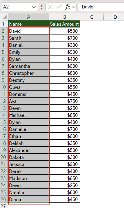
STEP 1: Highlight the range where you want to apply conditional formatting.

STEP 2: Go to the ‘Home’ tab and select ‘Conditional Formatting’ > ‘New Rule’.

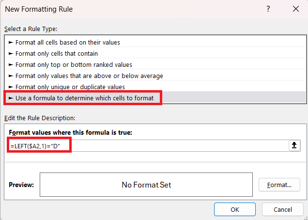
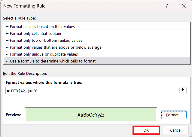
STEP 3:Select ‘Use a formula to determine which cells to format’. Then, in the displayed formula field, enter the criteria for your highlighting.

=LEFT($A2,1)=”D”

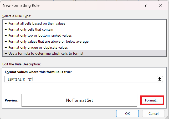
STEP 4: Press ‘Format’ button.

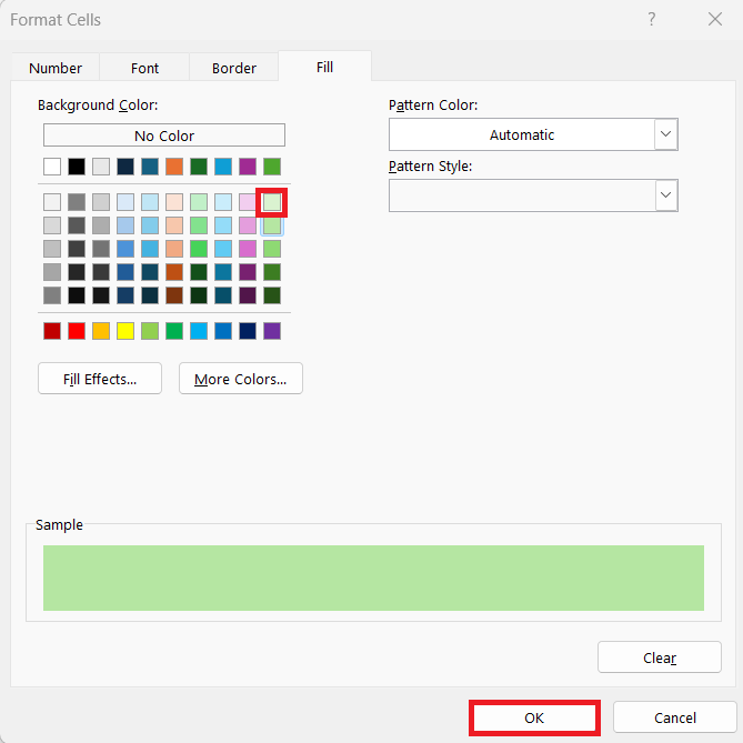
STEP 5: In the dialog box, navigate to the fill tab and choose a light green shade. Press OK.

STEP 6: Press OK.

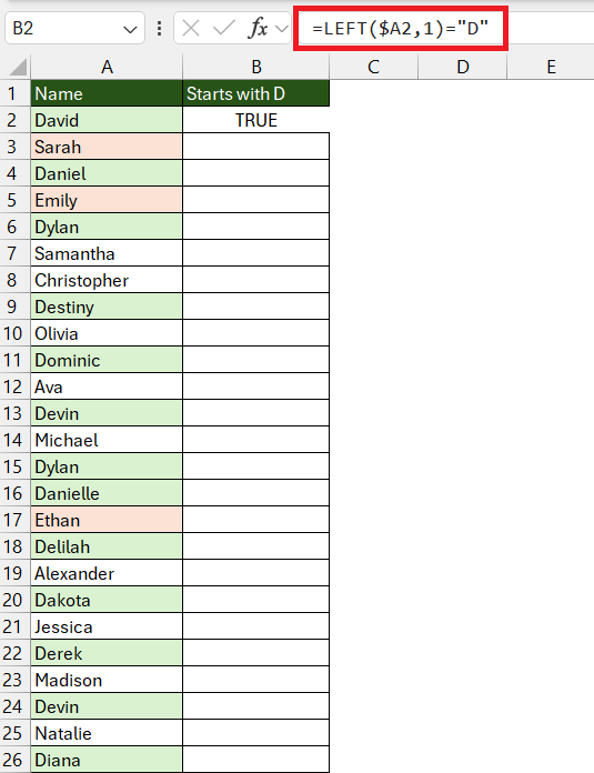
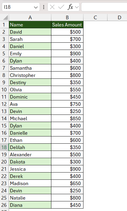
You can see that all the cells that start with the letter d have been highlighted.

 

Advanced Tips for Conditional Formatting

Manage Multiple Rules for Conditional Formatting

When dealing with multiple rules, it’s essential to keep things organized. Each rule in Excel is independent, but they can overlap. That’s why managing the order of precedence becomes important.

By following these steps, you can add another conditional formatting rule to check the text’s length and highlight rows that start with d in Excel. This allows for more comprehensive data highlighting based on multiple criteria.

STEP 1: Choose the range to which you wish to apply conditional formatting.

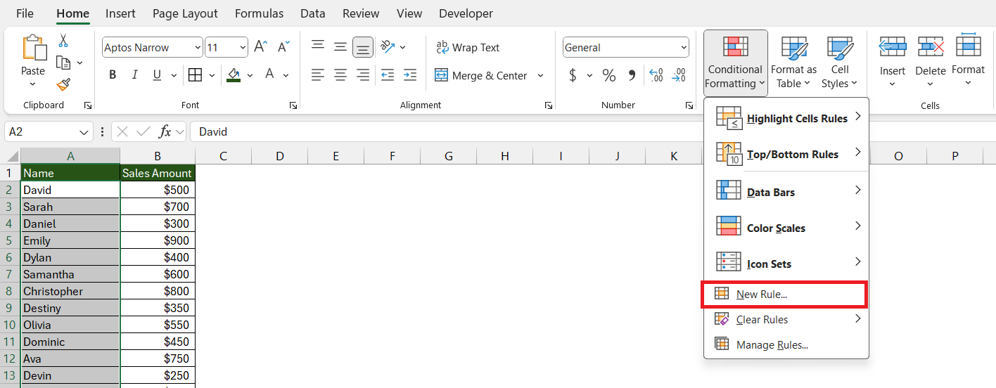
STEP 2:In your Excel workbook, navigate to the ‘Home’ tab. Choose ‘Conditional Formatting’ and then pick ‘New Rule’ from the dropdown list.

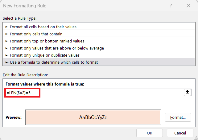
STEP 3: Click on ‘Use a formula to determine which cells to format’.Input the criteria for your highlight in the field.

=LEN($A2)=5

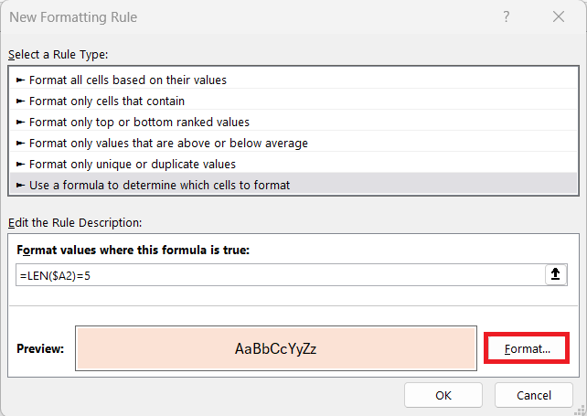
STEP 4: Press ‘Format’ button.

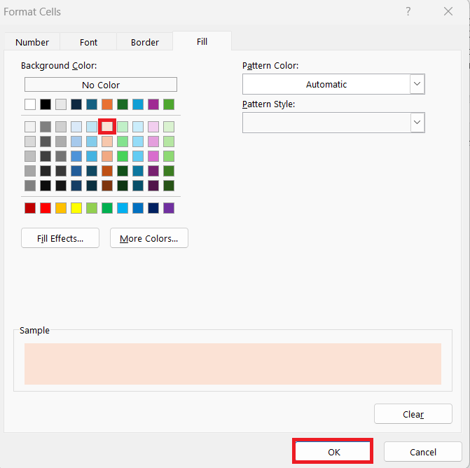
STEP 5: In the dialog box, navigate to the fill tab, choose a light red shade, and click OK.

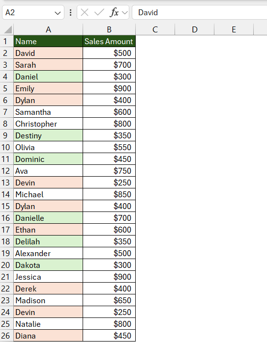
The rules are applied in the order they are listed in the Rules Manager, and you can change this order to suit your needs. You can see that in cell A2 even though the name starts with d, the cell is highlighted in red color. This is because the rule to check the length is above the rule to check the first letter.

If one rule contradicts another, the higher rule takes precedence. If they don’t contradict, both rules can apply, layering their effects.

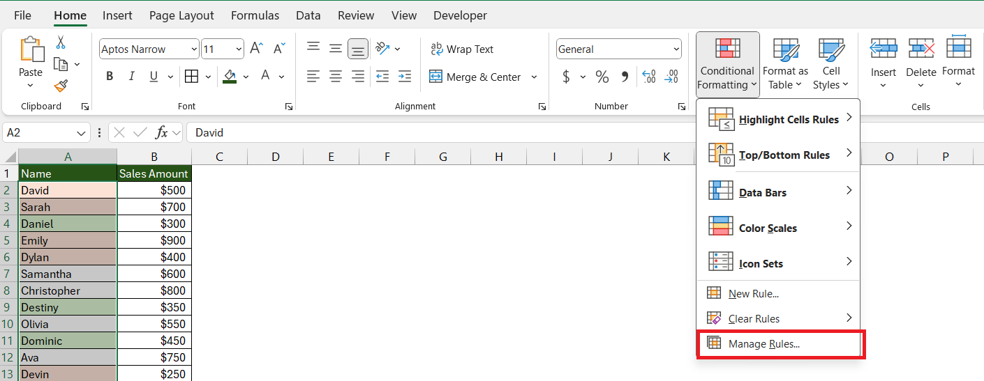
To avoid conflicts or unexpected results, regularly review your rules in the Conditional Formatting Rules Manager, which is accessible through the ‘Manage Rules’ option in the Conditional Formatting dropdown menu.

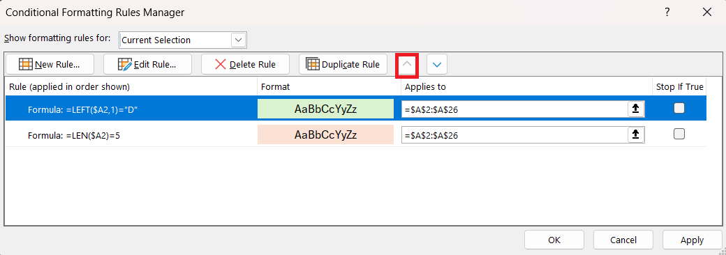
You can click on the small up arrow to move the rule to check the first letter at the top.

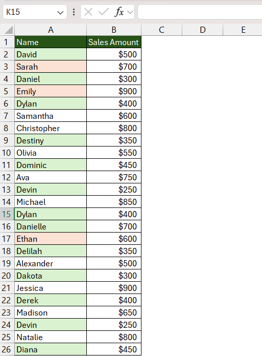
You can see that even though the length of the text in cell A2 is 5, the cell fill color is green because the rule to check the first letter is above the cell to check the length in the Conditional Formatting Rules Manager dialog box.

 

Ensuring Flexibility and Scalability in Formulas

Ensuring your conditional formatting formulas are both flexible and scalable is key for efficient data management as your Excel workbook grows. Flexible formulas adapt to changes in your dataset, like added rows or columns, without requiring constant updates. Scalability means that the formulas work just as well for 10 rows as they do for 10,000.

To achieve this, use absolute and relative cell references wisely. Generally, lock the column reference but leave the row reference relative (e.g., $A1 instead of $A$1) for row-based conditions. Additionally, base your formula on cell values instead of fixed criteria when possible, so that your rules dynamically adjust to the content.

 

Troubleshooting Common Issues

Handling Errors and Inconsistencies in Conditional Formatting

Errors and inconsistencies in conditional formatting can be baffling, but they’re not without solutions. First, make sure your formulas are correct and free from typos. Use Excel’s auditing tools to trace precedents and dependents to ensure all references are correct. Also, check for extra spaces and non-printing characters, as they can throw off text-based conditions.

When errors persist, use the ‘Clear Rules’ feature to remove formatting and start fresh. It’s also worth checking whether the range references are moving (relative) when they should be static (absolute). For instance, copying and pasting cells could change the range your rules apply to unintentionally.

Always test your rules with simple data and dummy formulas to isolate issues and remember to update and manage your rules, so they don’t conflict or become redundant.

FAQ Section

How do I apply conditional formatting to multiple rows?

To format multiple rows with conditional formatting, choose the row range you intend to format. Then, go to the ‘Home’ tab, click ‘Conditional Formatting’, and choose the rule that fits your criteria or create a new custom rule. Your formatting will apply to the entire range you’ve selected. Remember, rules are based on each cell in the specified range, so ensure your formula or condition reflects this.

What formula can be used to highlight rows that start with d?

You can use the following formula to highlight rows that start with D in Excel:

=LEFT(A1,1)=”D”

This formula checks if the first character in cell A1 (adjust the cell reference as needed for your data) is “D”. If it is, the condition is true, and the conditional formatting will be applied to that row.

What if my row starts with a lowercase ‘d’ instead of uppercase ‘D’?

This function can be used to check the first letter of the contents of the cell. The result will be case insensitive. Whether the first letter is ‘D’ or ‘d’, the result will be TRUE.

=LEFT(A1,1)=”D”

Can I highlight entire rows based on another column’s value?

Yes, you can highlight entire rows based on another column’s value by using conditional formatting with a custom formula. For example, if you want to highlight rows where Column B’s value is “Approved,” your formula would be:

=INDIRECT("B"&ROW())="Approved"

Apply this formula to the row range you want to format, and Excel will highlight the full rows corresponding.

How do I delete or alter an existing conditional formatting rule?

To remove or modify an existing conditional formatting rule, follow these steps:

• Select the cells where the rule is applied.
• Go to the ‘Home’ tab and select ‘Conditional Formatting’. Then choose ‘Manage Rules’ to view all the rules applied to the selected cells.
• Select the rule you wish to change or remove. To change it, edit the details and press ‘Apply’, or to remove it, hit ‘Delete’ and then ‘OK’ to confirm.