3 Easy Methods to Create Button in Excel for Macros

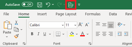
Do you repeat various Excel actions like copy & pasting data, formatting, putting borders, etc? Do you know that you create button in Excel and automate your tasks in Excel with a couple of mouse clicks? If you keep on repeating the same thing over and over again, creating an Excel Macro is perfect for you.  It saves you time so you can do things that you like doing, like going home early. Click a button and all your tasks are done for you. I will show you 3 different ways using which you can enable the Macro Creation and create button in Excel.

Key Takeaways

• ActiveX Control Buttons for Advanced Functionality: ActiveX control buttons provide a professional and customizable way to execute macros. They allow detailed adjustments such as font, size, and color customization directly in the worksheet.
• Quick Access Toolbar for Accessibility: Adding a macro button to the Quick Access Toolbar lets you run macros quickly from any worksheet. This method ensures accessibility without modifying the worksheet layout.
• Shapes as Flexible Buttons: Using shapes for macro buttons offers flexibility in design and placement. You can insert any shape, style it, and assign a macro to it, making it visually appealing and easy to integrate with your worksheet.
• Ease of Assigning Macros: Regardless of the method, Excel allows simple assignment of macros to buttons or shapes via the right-click menu. This ensures all methods are beginner-friendly and efficient.
• Customizable Options for Diverse Needs: Each method caters to different user needs—ActiveX for advanced functionality, the Quick Access Toolbar for convenience, and shapes for aesthetic customization—making it easy to choose based on your workflow.

Using ActiveX Control Buttons

Running a macro can sometimes be a tedious task. The fastest way to run a macro will be to assign a macro to a button. You can use ActiveX controls to create button in Excel.

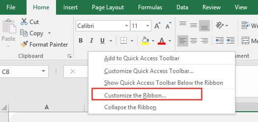
STEP 1: Right-click anywhere on your Ribbon and select Customize the Ribbon:

 

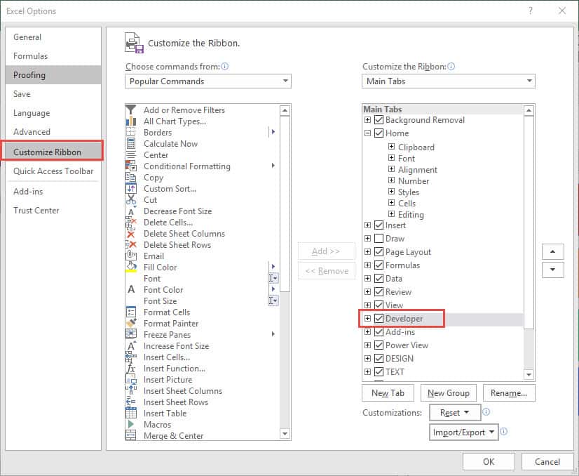
STEP 2: Make sure the Customize Ribbon is selected.

Then select the Developer option under Main Tabs.

Click OK.

 

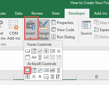
STEP 3: Now go to Developer > Insert > ActiveX Controls > Button

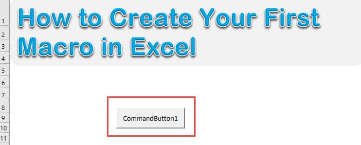
Drag anywhere in the Excel spreadsheet to create button in Excel.

 

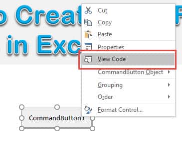
STEP 4: Right-click on your new button and select View Code.

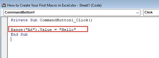
STEP 5: Type in this code:  Range(“A6”).Value = “Hello”

What this will do is to set the value of cell A6 to Hello.

 

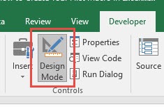
STEP 6: Time to test it out! Make sure Design Mode is deselected.

 

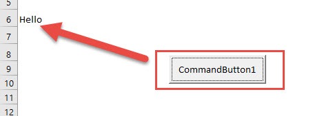
STEP 7: Click on the button now and you will see Hello pop up on your screen!

 

In this way, you can create button in Excel and assign a macro to it. Using VBA codes, you can also assign a different task for a different trigger like double-click single-click, right-click, etc.

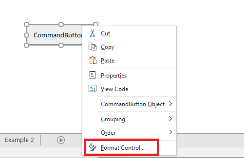
You can even change the formatting of this button by right-clicking on the button and selecting the option Format Control.

But the only issue with this method is that the size of the button may change when you make changes to the worksheet or share it with someone else.

 

Using Shapes

Shapes provide you the flexibility to format and customize the appearance of the buttons on your Excel spreadsheet.

You can use different shapes, icons, WordArt images, and objects as per the theme of your worksheet. The formatting will also remain consistent using this method.

In my opinion, this is the simplest and most adaptable option to create button in Excel and run a macro.

 

Let’s look at a detailed tutorial on how we can go about this:

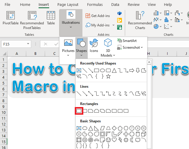
STEP 1: Go to Insert Tab > Select Illustrations > Under shapes dropdown > Select rectangle shape.

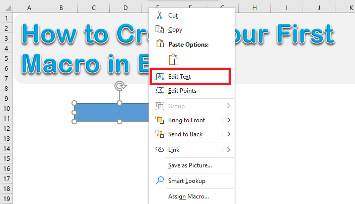
STEP 2: Right-click the shape and select Edit Text to add text to the button.

Or, you can double click on the button to edit text.

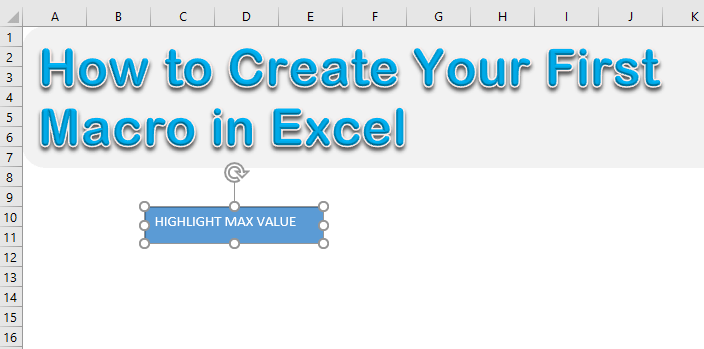
STEP 3: Provide a name to this button – Highlight Max Value.

STEP 4: Go to Developer >Visual Basic.

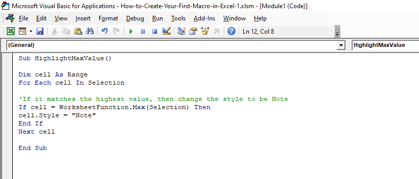
STEP 5: Type the following code in the module.

Copy Source Code:

Sub HighlightMaxValue()

Dim cell As Range
For Each cell In Selection

'If it matches the highest value, then change the style to be Note
If cell = WorksheetFunction.Max(Selection) Then
cell.Style = "Note"
End If
Next cell

End Sub

HighlightMaxValue will now be saved!

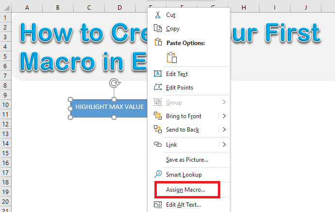
STEP 6: You can easily add a macro to this button by right-clicking on the button and select Assign Macro.

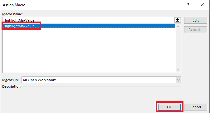
STEP 7: In the Assign Macro dialog box, you can select one macro (here, HighlightMaxValue) from the list saved in the Excel Workbook. Click OK.

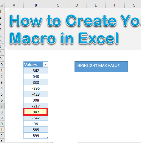
This HighlightMaxValue will highlight the cell with maximum value with yellow color.

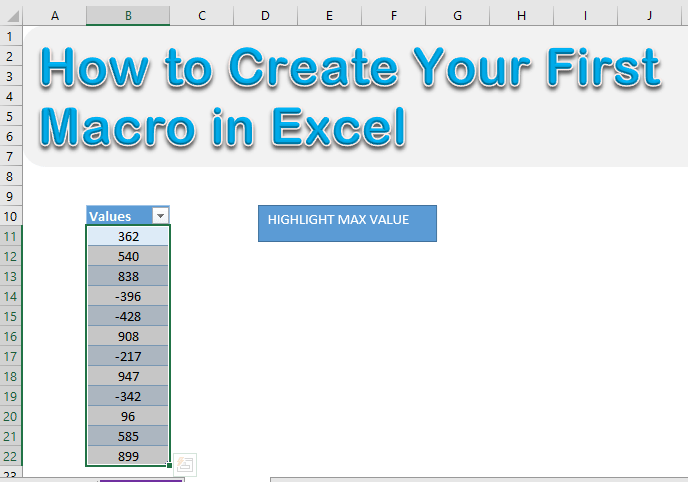
STEP 8: Select the range and then press the Excel Macro button.

STEP 9: Select the maximum value from the range i.e. 947 will be highlighted.

This is how you can easily use shapes to create button in Excel and assign a macro to it.

 

You can also customize these buttons by following the steps below:

• Hold the Ctrl key and click on the button.
• Go to Shape Format Tab
• Select an appropriate option from the list – shape fill, shape outline, shape effects, text fill, text outline, text effects, size, etc.

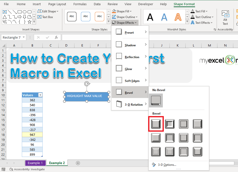
To provide the button a 3-D effect – Go to Shape Format > Shape Effects > Bevel > Round.

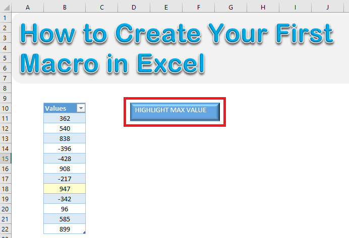
This is how your 3-D Excel Macro button will look like:

 

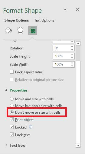
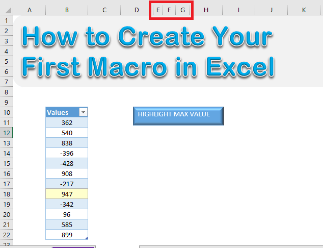
You can also prevent these buttons from changing their size when you change the size of a column or row.

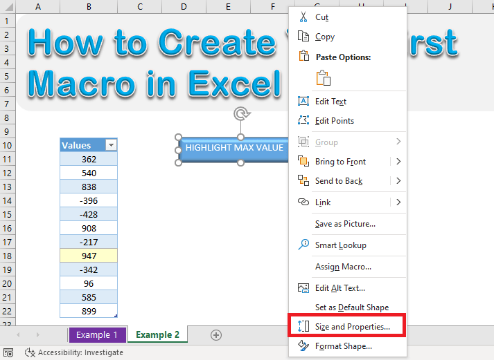
• Right-click on the button and select Size and Properties.
  
• In the Format Shape dialog box, go to Properties and select Don’t move or size with cells.
  

Now, even if you change the size of the rows or columns, the button will remain intact.

Add to Quick Access Toolbar

You can easily add a macro as a button on the Quick Access Toolbar and use it on any of the sheets present in the workbook.

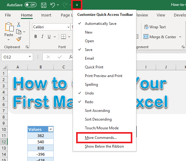
STEP 1: Right-click on the arrow next to the Quick Access Toolbar and select More Commands.

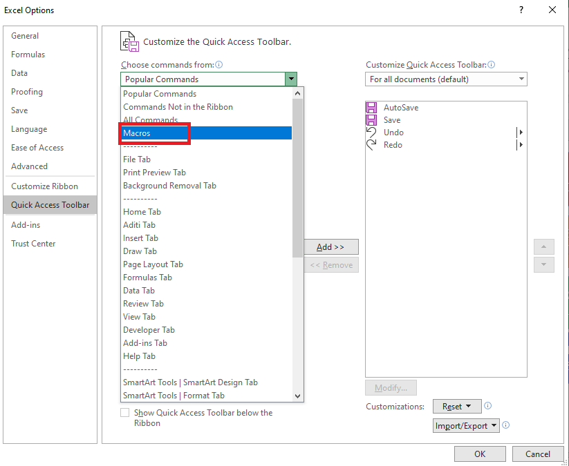
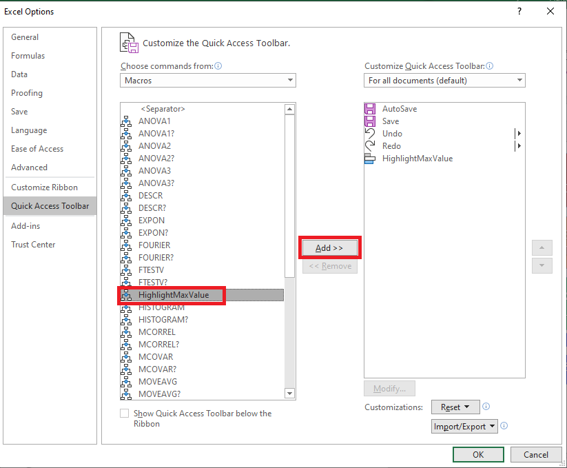
STEP 2: In the Choose commands from list, select Macros.

STEP 3: Select HighlightMaxValue from the list and click on Add>>.

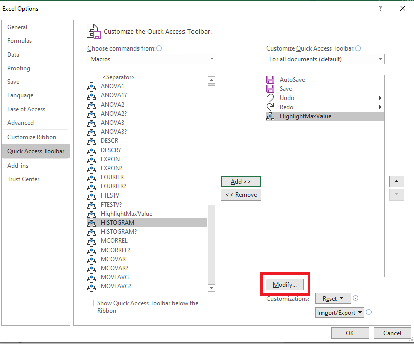
STEP 4: Click on Modify to change the symbol of this macro.

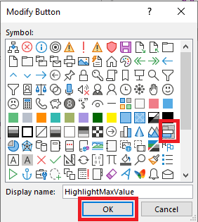
STEP 5: Select an appropriate symbol and click OK.

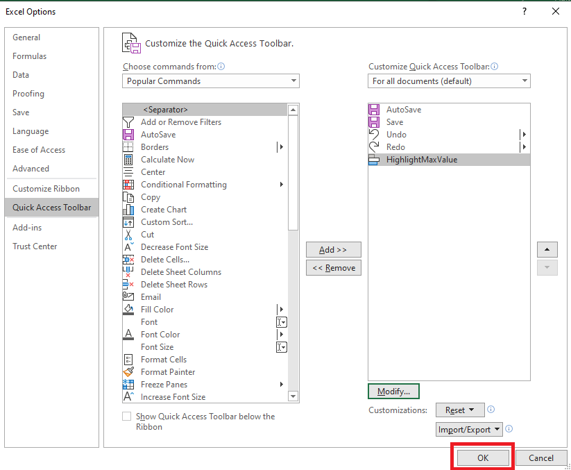
STEP 6: Click OK.

 

Your Quick Access Toolbar will now contain the macro – HighlightMaxValue. Simply, click on this icon and your macro will run!

Frequently Asked Questions

How can I create a button using ActiveX controls in Excel?
To create an ActiveX control button, go to the Developer tab and click Insert. Select the ActiveX Command Button and draw it on your worksheet. Then, right-click the button, select Properties to customize it, and assign a macro by choosing Assign Macro from the context menu.

How do I add a macro to the Quick Access Toolbar?
To add a macro to the Quick Access Toolbar, click the dropdown arrow on the toolbar (usually at the top of the Excel window), select More Commands, and switch the dropdown menu to Macros. Choose your macro, click Add, and customize its icon and label before saving.

Can I use shapes as buttons to run macros?
Yes, you can use shapes as buttons. Insert a shape from the Insert tab, customize it with colors or text, and right-click to select Assign Macro. Choose the macro you want to link, and clicking the shape will execute the assigned macro.

What is the difference between ActiveX buttons and shapes for macros?
ActiveX buttons offer more advanced customization options, like modifying font, size, and properties programmatically. Shapes are simpler to use and more flexible for design purposes, but they don’t have as many built-in features as ActiveX buttons.

Which method is best for creating a button in Excel?
The best method depends on your needs. Use ActiveX buttons for advanced functionality and customization, the Quick Access Toolbar for easy access across worksheets, and shapes for visually appealing and creative designs within the workbook.