How to Find the Maximum Value with Max Function in Excel

Finding the maximum value in Excel is a quick and easy way to identify the largest number in a range of data. Whether you’re analyzing sales figures or tracking performance, Excel offers several methods, such as using the MAX function or applying conditions with MAXIFS, to get the highest value efficiently. Let me guide you through the process step-by-step on how to find the maximum value in Excel.

Key Takeaways:

• Use the MAX function to quickly find the largest number in a range of data.
• Apply MAXIFS when you need to find the highest value based on specific criteria.
• The MAX function can handle fixed, non-adjacent, and row/column ranges effortlessly.
• Use functions like IFERROR to manage errors within ranges for smooth MAX calculations.
• From sales assessments to student scores, the MAX function is widely applicable in various industries.

 

Unlocking Excel MAX Function Basics

Defining the MAX Function in Excel

The MAX function is a powerful tool in Excel’s arsenal, specifically designed to help us find the highest number in a list of values. Whether dealing with sales data, exam scores, or any numerical set, we rely on MAX to sift through the information and declare the winner – the top value.

Navigating Through the Syntax and Arguments

To use the MAX function correctly, we need to understand its syntax: MAX(number1, [number2], ...). The first argument, number1, is mandatory, and we can include up to 254 additional numbers, which are optional.

These numbers can be constants, cell references, formulas, or even range names. I appreciate the simplicity: we just need to feed it numbers, and it diligently reports back with the biggest one.

 

Step-Up Your Excel Game: Applying MAX

Simple Steps to Create a MAX Formula

Creating a MAX formula is straightforward, even if we’re not spreadsheet savants. I like to think of it as telling Excel, “Hey, show me the big guy in this lineup.” So, here’s what we do:

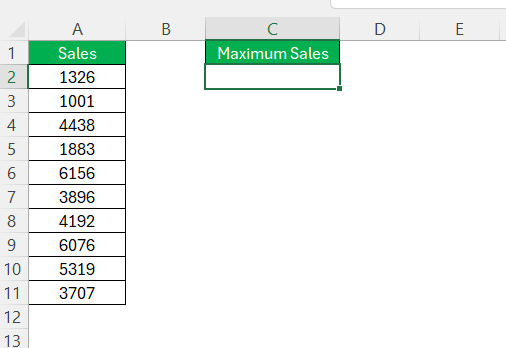
STEP 1: Click on the cell where the maximum value should be displayed.

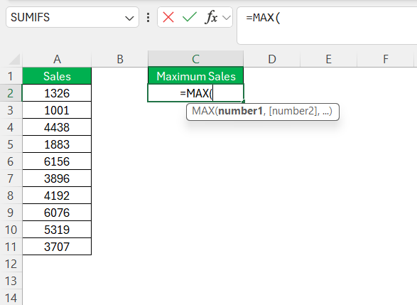
STEP 2: Type =MAX( to initiate the function.

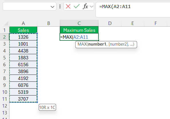
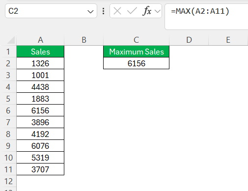
STEP 3: Select the range of cells with the mouse or type them manually, like A2:A11.

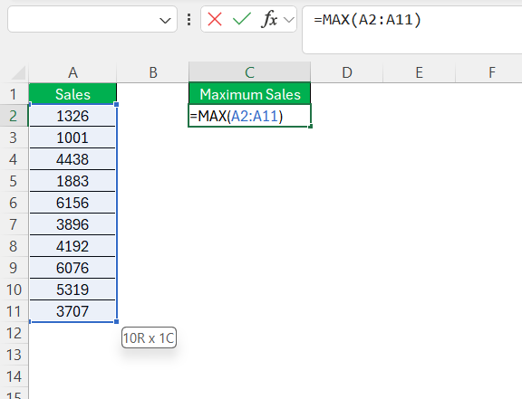
STEP 4: Close the function with a parenthesis – ).

STEP 5: Hit the Enter key, and like magic, the highest value in the range appears.

It’s a smooth process that turns columns of numbers into a single, highest-value reveal.

Breaking Down Formula Variations and Scenarios

The MAX function can be tailored to different scenarios. Here are a few formula variations to consider:

• Current Row/Column: To find the maximum in the current row or column, use =MAX(1:1) or =MAX(A:A).

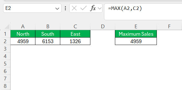
• Fixed Range: Lock onto a fixed range with absolute references, like =MAX($A$1:$A$10).
• Non-contiguous Range: For non-adjacent cells, combine them by commas: =MAX(A2, C2).

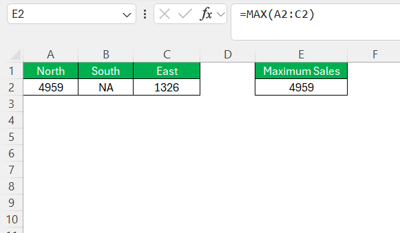
• Including Text: If a range includes text or logical values, MAX will ignore them automatically.

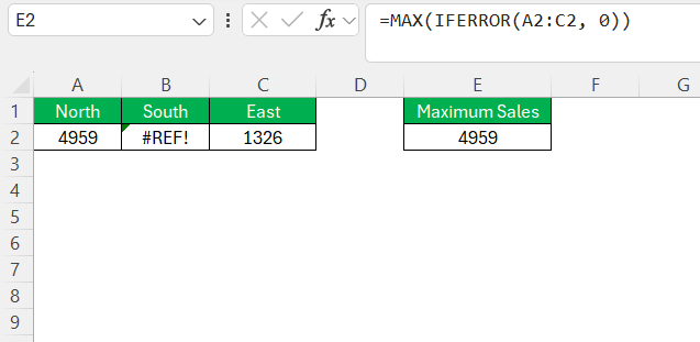
• Handling Errors: Combine with IFERROR to manage errors within data: =MAX(IFERROR(A1:A10, 0)).

Whatever our data looks like, we can flex MAX to fit. It’s like having a range of lenses to focus precisely on what we need.

 

Overcoming the Common Hurdles with MAX Function

Solutions for Frequent Errors with MAX Formulas

We’re bound to hit some snags with MAX formulas. Here are a few solutions to common errors:

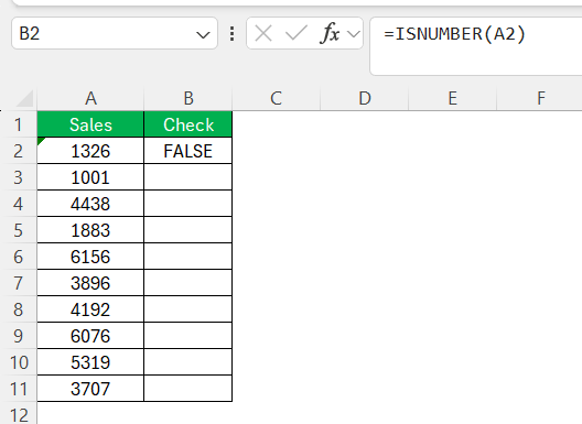
• Text-formatted Numbers: If MAX returns 0 when it shouldn’t, check if the numbers are actually text. Use =ISNUMBER(A1) to confirm. If false, they’re text and need conversion.

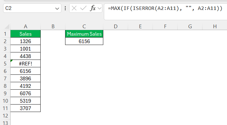
• Errors in Data: If a cell in the range contains an error, MAX will too. Use =MAX(IF(ISERROR(A2:A11), "", A2:A11)) to exclude errors.

• Hidden Zeros: Sometimes, “invisible” zeros affect the result. If we’re certain values should be ignored, they need to be removed or replaced.

It’s like troubleshooting a car – a bit daunting at first, but with the right tools, we get it purring again.

Expert Tips for Dealing with Non-Contiguous Cells and Ranges

Getting the MAX from non-contiguous cells and ranges can trip us up, but I’ve got some pro tips:

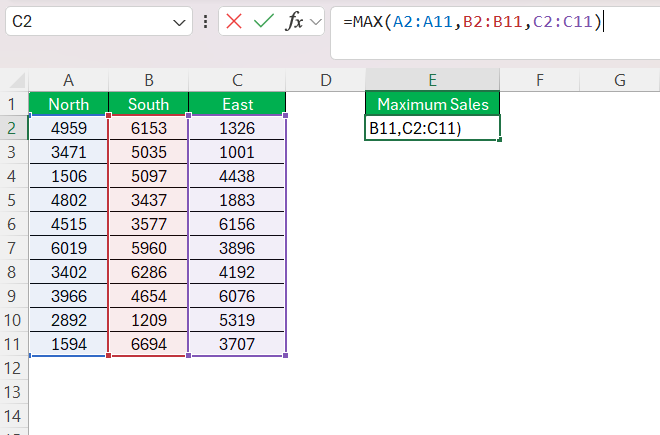
• Ctrl-Click Selection: While typing =MAX(, hold Ctrl and click each cell or range. Excel compiles these into a formula like =MAX(B2, D2:F2, H2).

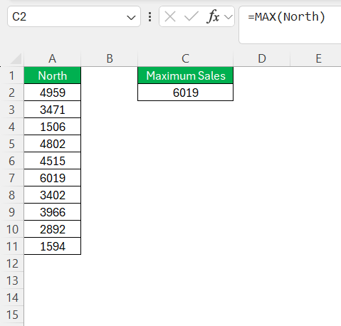
• Named Ranges: Define cells as a named range. This keeps things tidy: =MAX(North).

Think of it as solving a puzzle—we’re piecing together separate data bits to see the big picture.

 

Advanced Excel Techniques: Beyond the Basic MAX

Unleashing MAX Function With Conditions

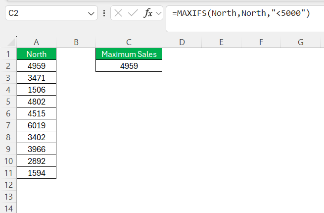
When we need the MAX function to get a bit more sophisticated and consider conditions, MAXIFS is our go-to. It’s MAX with a detective’s hat, sleuthing through rows and identifying the highest value that meets our specific criteria. We construct it as MAXIFS(max_range, criteria_range1, criteria1, [criteria_range2, criteria2],...).

This version does more than just pick the biggest number—it eyes our dataset with a set of conditions in hand, ensuring that only the most relevant values count. Say we’re hunting for the highest sales but only in a particular region. We’d set up MAXIFS to consider the sales numbers, but only where cells in the region column match our target area.

How to Find and Highlight the Max Value in Data Sets

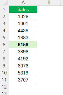
To spot the big fish in our data sea, I like to use conditional formatting together with the MAX function. Here’s the drill:

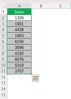
STEP 1: Select the data range you’re eyeing for the maximum value.

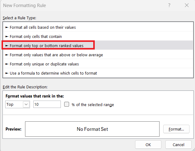
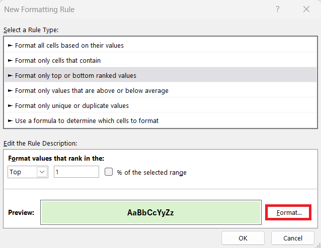
STEP 2: Navigate to the Home tab, click on ‘Conditional Formatting’, and choose ‘New Rule’.

STEP 3: Pick ‘Format only top or bottom ranked values’.

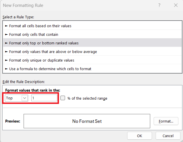
STEP 4: Set the rule to format cells that rank within the top 1.

STEP 5: Apply the format of your choice – make it bold, change the font color, or fill the cell with color.

The effect is immediate: our max value stands out, visually flagged for easy identification, amidst a sea of numbers.

 

Real-world Examples: MAX in Action

Case Studies of MAX Function Solving Business Problems

In the business realm, the MAX function often plays the hero, solving problems with a flourish. Here are a couple of inspiring case studies:

• Sales Data Assessments: Imagine a company facing a plethora of product sales numbers. With MAX, they pinpointed the product with the highest sales, leading to focused marketing strategies that boosted revenue.
• Financial Forecasting: A finance team used MAX to identify peak spending in historical data, helping to forecast budgets and cut costs where needed.

These are glimpses of MAX as more than a mere function – it’s a decision-making ally, turning heads in the meeting room when it counts.

Creative Uses of MAX Function in Different Industries

The MAX function’s adaptability across sectors is kind of like a Swiss Army knife – versatile and dependable. Here are some creative industry-specific uses:

• Education: Teachers use MAX to find the highest score in a test, providing instant recognition for top performers and setting benchmarks for the class.
• Healthcare: Analysts apply MAX to patient data to determine peak health statistics or critical levels that require intervention.
• Retail: Store managers leverage MAX to recognize their highest-selling items or peak shopping hours, informing stock decisions and staffing.

Whether it’s the crest of academic achievement or the pinnacle of heart rates, MAX peeks through the data looking for those summits.

 

FAQs: Mastering MAX in Excel

How to find the maximum value of a function?

To find the maximum value of a function in Excel, use the MAX function. Enter =MAX(range) where “range” is the set of cells containing the function’s output. Excel then scans these values and delivers the highest one. It’s efficient for summarizing complex data calculations with a high-point focus.

Why Does My MAX Formula Return an Error?

If your MAX formula returns an error, it’s likely because there’s an error value within your data range. Excel’s MAX function will return an error if even one cell in the range has an error. To resolve this, use =MAX(IF(ISERROR(your_range), "", your_range)) to ignore the errors.

How Can I Make a MAX Function Ignore Zeros?

To make the MAX function ignore zeros, combine it with the IF function: =MAX(IF(your_range <> 0, your_range)). Remember to press Ctrl+Shift+Enter if you’re not using Excel 365, as it’s an array formula. This tells Excel to only consider non-zero numbers as contenders for the maximum value.

What Is the Best Way to Find the Maximum Value in Non-Adjacent Cells?

The best way to find the maximum value in non-adjacent cells is using the MAX function with cell references separated by commas. For example, =MAX(A2, C2, E2). Alternatively, for non-adjacent ranges, use =MAX(range1, range2, range3,...). This methodology ensures you target only the cells you’re interested in.

How do I find the maximum value in Excel using criteria?

Finding the maximum value in Excel using criteria involves using the MAXIFS function or an array formula. With MAXIFS, you specify the range to find the max from, alongside one or multiple criteria. For example, =MAXIFS(max_range, criteria_range1, criteria1). For an array formula, use =MAX(IF(criteria_range1=criteria1, max_range)) and remember to press Ctrl+Shift+Enter if you’re not working in Excel 365.