How to Freeze Rows in Excel – Step by Step Guide

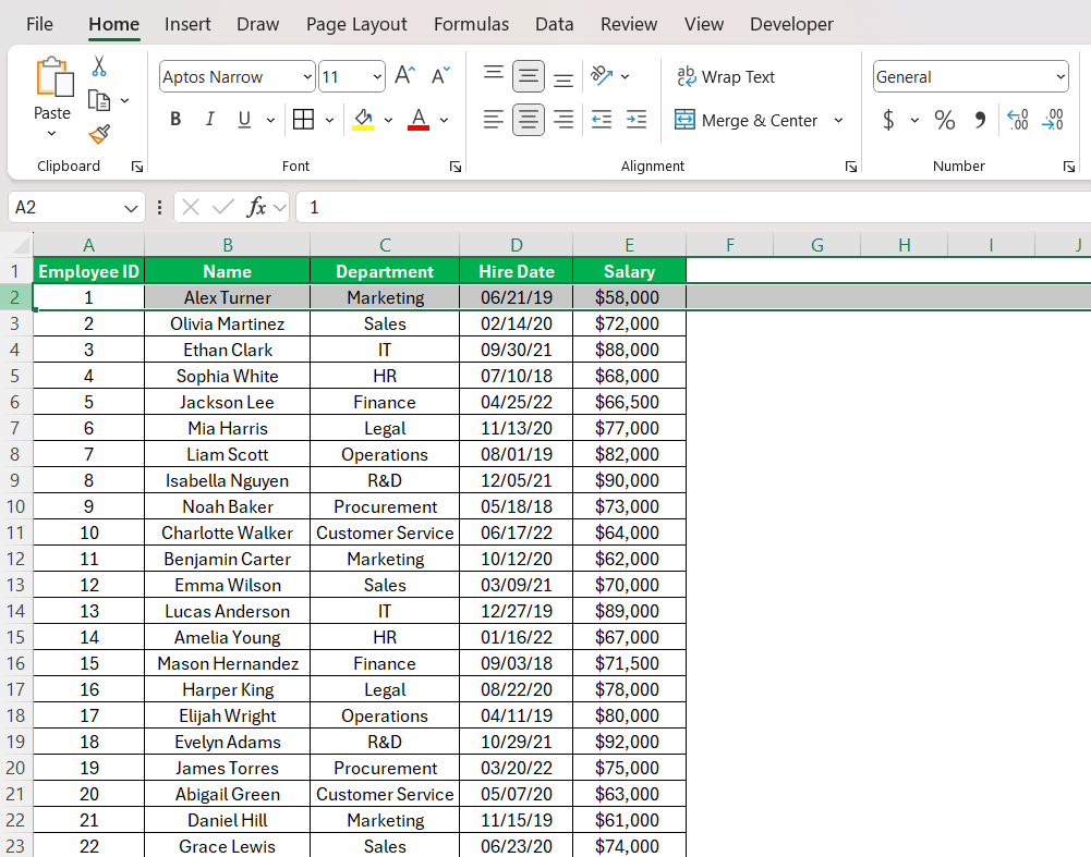
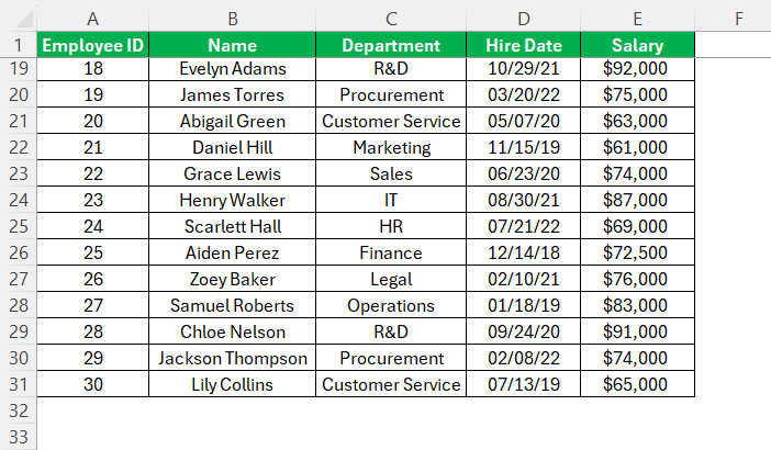
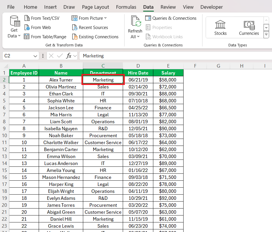
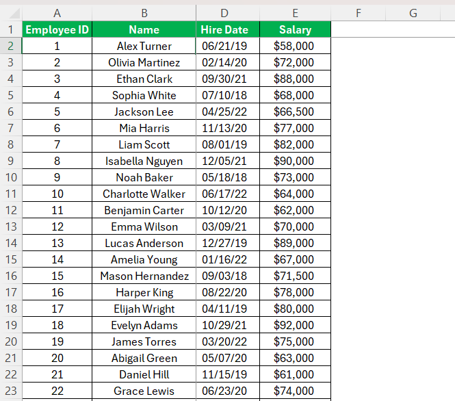
When working with large datasets in Excel, it can be challenging to keep track of important headers or labels as you scroll through your worksheet. I often find myself losing sight of crucial information, which can slow down my work. Freezing rows in Excel is a simple yet powerful feature that ensures your key data stays visible, no matter how far you scroll. In this article, I’ll guide you through the steps on how to freeze rows in Excel so you can keep your work organized and efficient.

Key Takeaways:

• Freezing rows in Excel keeps important headers visible while scrolling through large datasets.
• The ‘Freeze Panes’ feature allows you to lock single or multiple rows and columns.
• Troubleshoot freezing issues by ensuring the selected rows are visible and removing filters or groupings.
• You can freeze both rows and columns simultaneously for enhanced data management.
• Keyboard shortcuts and the Quick Access Toolbar can speed up the process of freezing and unfreezing panes.

 

Introduction to Data Management in Excel

The Importance of Freezing Rows

Managing data in Excel can be overwhelming, especially when dealing with extensive datasets. This is where freezing rows come into play. I’ve noticed that by fixating specific rows, such as headers, on the screen, one can keep vital information readily available despite scrolling through the spreadsheet.

This ensures that I don’t lose track of which data belongs to which category, facilitating accuracy and efficiency alike.

Applications in Everyday Excel Use

In my everyday use of Excel, freezing rows has a wide range of applications. It’s an indispensable tool during tasks like data entry, as it allows me to maintain a point of reference. When analyzing financial reports or datasets, headings remain visible, ensuring that I constantly have the contextual information needed for accurate interpretation.

Similarly, if I’m compiling a list that spans numerous entries, freezing the top row with column names keeps me from getting lost in the sea of data.

Frequently, project managers and administrators utilize this feature to track project timelines and task ownership without losing sight of the headers as they delve into the details. This level of organization and accessibility offered by Excel is crucial for productivity and data management efficiency.

 

Step-by-Step Guide on How to Freeze Rows in Excel

Using ‘Freeze Panes’ to Lock Single or Multiple Rows

Freezing rows in Excel is straightforward. I ensure that the headers or rows I want to keep in view are at the top of my spreadsheet, then navigate to the ‘View’ tab. Under this tab, there’s an option called ‘Freeze Panes’. Here’s the simple process I follow:

STEP 1: Position the cursor in the cell immediately below the row I wish to freeze.

STEP 2: Click on ‘View’, and within this tab, find and select ‘Freeze Panes’.

STEP 3: Choose ‘Freeze Top Row’ to lock the first row. If I want to freeze more than one row, I use the ‘Freeze Panes’ option instead.

By following these steps, I can keep selected rows in place while the rest of the spreadsheet scrolls freely, which is particularly handy for comparing figures located in different sections of the document.

Troubleshooting Common Issues When Freezing Rows

While the process of freezing rows is generally seamless, I’ve come across some issues that can prevent it from working correctly. If you can’t freeze rows, it might be due to the selected row not being visible — Excel requires the row to be onscreen to freeze it. I make sure to scroll to the row before attempting the feature.

Another stumbling block can be existing filters or grouping on the worksheet. Since these alter how rows are displayed, they might conflict with freezing panes. I’ve found that removing these filters or groupings temporarily allows for the freezing action to be successful.

A less common but possible hindrance is using an outdated or limited Excel version, as not all support freezing panes. Upgrading to the latest version often resolves this issue.

 

Advanced Tips for Freezing Rows

Freezing Columns and Rows Simultaneously

Freezing both columns and rows simultaneously is a fantastic capability in Excel that further enhances data management. Here’s how I approach this:

STEP 1: First, I identify the rows and columns that need to stay fixed on the screen. Select the cell that is immediately below and to the right of the rows and columns I want to freeze. For instance, if I need to freeze the first row and the first 2 column, I select cell C2.

STEP 2: Then, I click ‘Freeze Panes’ under the ‘View’ tab.

By using this feature, both the column to the left of the cell and the rows above it are locked in place.

It’s particularly helpful in maintaining the visibility of both row headers and column labels simultaneously, which is a boon during data analysis and comparison tasks.

 

Utilizing Keyboard Shortcuts for Efficiency

To breeze through data management tasks, I rely heavily on keyboard shortcuts. While there is no direct shortcut for freezing panes, a combination can achieve the result swiftly:

• For Windows, I press Alt + W + F + F and then hit Enter. It quickly activates the Freeze Panes feature, allowing me to lock rows or columns without reaching for the mouse.
• On MacOS, I use Command + Option + 0 to accomplish the same goal.

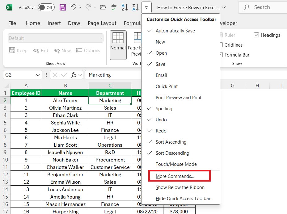
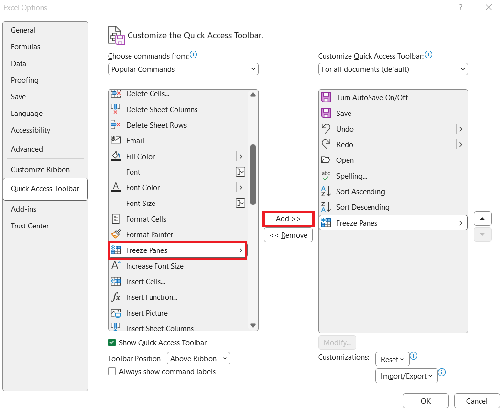
Moreover, adding Freeze Panes to the Quick Access Toolbar is a power move. It lets me freeze or unfreeze panes with just a click, bypassing the ribbons altogether. I simply click the small dropdown arrow on the toolbar and select “More Commands”.

In the dialog box, select “Freeze Panes” from the “Popular Commands” list and click on “Add”.

And it’s set.

 

Unfreezing Panes for Flexible Data Analysis

How to Properly Unfreeze Panes in Excel

Unfreezing panes in Excel is a clear-cut process but vital to restoring full movement across the spreadsheet. Here’s what I do:

After navigating to the ‘View’ tab, I locate the ‘Window’ group. Then, a simple click on the ‘Freeze Panes’ button followed by selecting ‘Unfreeze Panes’ from the dropdown swiftly relinquishes any fixed rows or columns.

It’s crucial to note that if the ‘Unfreeze Panes’ is greyed out, it indicates there are currently no panes frozen on the active worksheet. Should there be a need to frequently toggle between frozen and unfrozen states, understanding this quick method is a huge time saver.

When to Toggle Between Frozen and Unfrozen Views

Switching between frozen and unfrozen views is all about the context of the task at hand. When I’m entering data or scanning through large datasets, freezing panes provide a static reference point which is crucial for accuracy. However, when I need to analyze data relationships or undertake a comprehensive review of the spreadsheet without headers blocking the view, unfreezing becomes necessary.

Moreover, when preparing to print, present, or share the spreadsheet, I toggle off the freeze to ensure the document appears as intended for the audience. Understanding when and how to toggle is a key skill that I find improves the versatility and usability of my Excel spreadsheets.

 

FAQs

Why can’t I freeze rows in my Excel worksheet?

You might not be able to freeze rows if the row isn’t visible, or you’ve scrolled away from the top. Also, filters or groupings on the worksheet can interfere, so removing them might help. If you’re in cell editing mode or your worksheet is protected, try exiting the mode or removing the protection. Lastly, ensure your Excel version supports freezing panes.

Can I freeze multiple rows and columns at the same time?

Absolutely, you can freeze multiple rows and columns simultaneously in Excel. To do this, simply select the cell below and to the right of the area you want to freeze. Then, go to the ‘View’ tab, click ‘Freeze Panes’, and select ‘Freeze Panes’ from the dropdown menu.

How do I freeze certain rows in Excel?

To freeze certain rows in Excel, select the row below the rows you want to freeze. Next, go to the ‘View’ tab, click on ‘Freeze Panes’, and then choose ‘Freeze Panes’ from the drop-down menu. Your selected rows above will now remain in view as you scroll through your worksheet.

What is the shortcut for freezing rows in Excel?

For freezing rows in Excel quickly, use the keyboard shortcuts. On Windows, press Alt + W + F + F and hit Enter, and on MacOS, use Command + Option + 0. This helps you immediately activate the Freeze Panes feature without navigating through the ribbon.

How can I freeze a column?

To freeze a column in Excel, select the column to the right of the one you want to freeze. Then go to the ‘View’ tab, choose ‘Freeze Panes’, and select ‘Freeze Panes’ again. This locks the column(s) to the left, keeping them visible as you scroll horizontally across your worksheet.