Unique values in your Excel spreadsheets can be a goldmine of insights, allowing you to uncover patterns and outliers that could inform your decisions and strategies. They help you to determine the frequency of specific values and can be particularly useful in quality control by ensuring data integrity through the identification of duplicates which, once removed, can lead to more accurate and reliable data analysis.
Key Takeaways:
- The UNIQUE function is an efficient tool to extract distinct values from a specified range in Excel, especially useful in the latest versions of Excel 365 that support dynamic arrays.
- An alternative to the UNIQUE function is the Remove Duplicates feature located in the Data tab, which allows users to delete any duplicate entries, leaving only unique values in a given range.
Table of Contents
Common Scenarios for Using Unique Values
Identifying unique values in Excel is multifaceted, catering to scenarios as diverse as data cleaning, statistical analysis, and customer segmentation. Educators might leverage unique scores for grading insights, while sales teams might track unique products bought to understand consumer behavior. In finance, ensuring transactions are recorded singularly is crucial to balance the books, and in marketing, identifying unique customer touchpoints can inform engagement strategies.
Mastering Unique Values with Excel Functions
Harnessing the Power of the UNIQUE Function
The UNIQUE function in Excel is your key to simplifying complex tasks of data analysis. With its ability to spill out an array of distinct values, you’ll no longer need to painstakingly comb through data for duplicates. Just enter =UNIQUE(range) into a cell and watch as Excel automatically populates adjacent cells with every one-of-a-kind value from your selected range. This function is a game-changer for those working with large datasets, saving time and enhancing productivity.
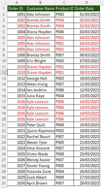
STEP 1: Find the data set that contains duplicate values
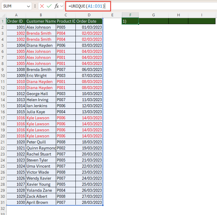
STEP 2: Type in the formula =UNIQUE(A1:D31)
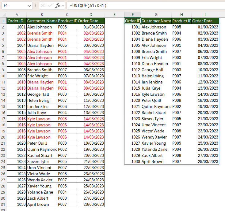
STEP 3: You will get all of the unique records in a new table!
Dynamic Arrays: A New Era of Data Management
Dynamic arrays in Excel are revolutionizing the way you manage data. They allow functions to return multiple results to a range of cells simply by writing a single formula. This method, introduced in Office 365, means formulas are smarter, more flexible, and efficient, doing away with the need for cumbersome workarounds like the Control-Shift-Enter array formulas of the past. This results in cleaner sheets and vastly improved workflow, especially when dealing with large datasets requiring unique entries.
Advanced Techniques for Unique Entries
Filtering Distinct Values Like a Pro
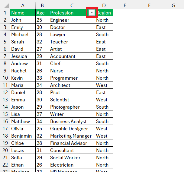
Filtering for distinct values in Excel allows you to separate the wheat from the chaff. You can achieve this quickly by using the built-in Filter feature. Simply select your range and head over to the Data tab to apply a filter. Then, tap on the drop-down arrow in the header row and select the items you wish to view. With this technique, managing and analyzing data becomes significantly more straightforward, enabling you to focus on the unique information you need.
Expert Use of Excel’s Advanced Filter
Excel’s Advanced Filter is a formidable tool that enables handling complex criteria with poise, especially when you need to extract unique records from a dataset. They make it possible to state conditions using formulas and support outputting the results to a different location, keeping your original data untouched. You might want to remember that to unlock this feature, clearly label each column header to avoid confusion. By selecting unique records only, one can extract unique rows too, helping you maintain clean, duplicate-free data.
Highlighting Your Data’s Uniqueness
Visual Cues: Identifying Unique and Distinct Rows
Adding visual cues to your Excel data can dramatically improve readability and error detection. Identifying unique and distinct rows is straightforward with conditional formatting. You can apply a color or a style to rows containing unique values, ensuring they stand out from the crowd. This instant visual feedback enables you to quickly spot patterns and anomalies in your dataset, turning a table full of numbers and text into a clear, organized canvas of data points.
Custom Rules for Highlighting Unique Values
Creating custom rules for highlighting unique values in Excel brings precision to your data management. With conditional formatting, a formula-based rule can specify exactly what you consider unique, considering the entirety of the row or specific columns. For instance, the formula =COUNTIF($A$2:$A$10, $A2)=1 will illuminate only those values that appear exactly once. Additionally, formulas like =COUNTIF($A$2:$A2, $A2)=1 can draw your attention to the first occurrence of every distinct value, empowering you with the ability to tailor your data visualization to your exact needs.
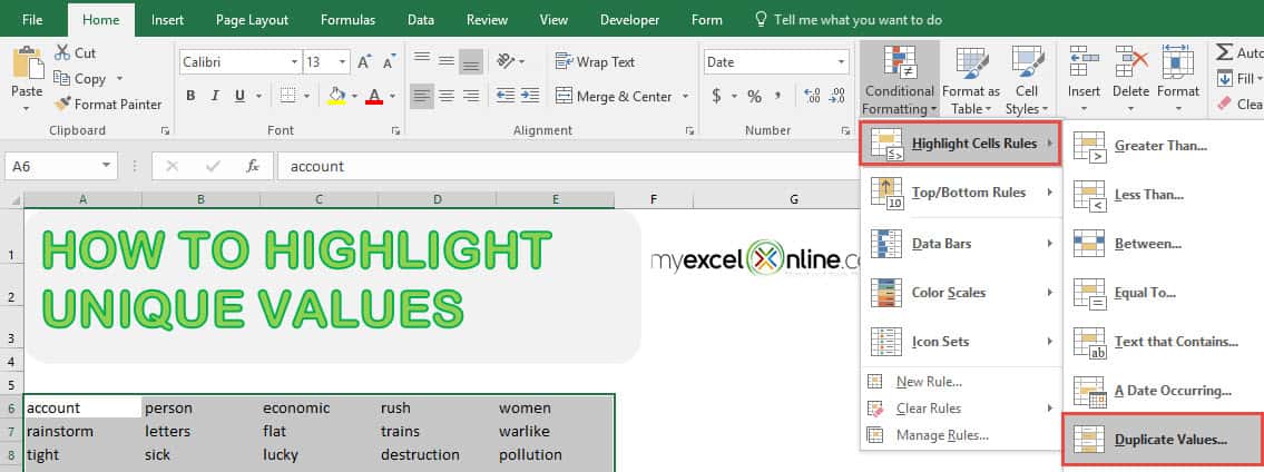
You can also use Conditional Formatting to highlight the unique values to identify them right away:
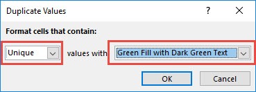
Make sure to select Unique.
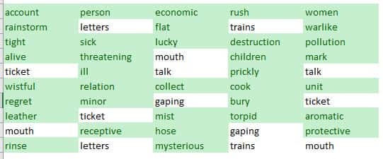
Then the unique values immediately get highlighted!
FAQs on Excel Unique Values
How Do I Generate a List of Unique Values from a Column?
To generate a list of unique values from a column in Excel, you can use the UNIQUE function. Simply enter =UNIQUE(range) in a cell, where “range” is the set of cells you’re interested in. This will return a list of distinct values from that range. For versions without the UNIQUE function, apply filters, or use the advanced filter to extract unique values to a different location.
Can Excel Automatically Highlight Unique Data?
Yes, Excel can automatically highlight unique data for you. Use conditional formatting by selecting your data, then go to ‘Home’ > ‘Conditional Formatting’ > ‘Highlight Cells Rules’ > ‘Duplicate Values’. In the dialogue box, switch from ‘Duplicate’ to ‘Unique’, select your formatting choice, and click OK.
What Are Dynamic Array Functions and How Do They Help with Uniqueness?
Dynamic array functions, like UNIQUE, FILTER, and SORT, output multiple values automatically and adjust in size when the source data changes. They help with uniqueness by efficiently returning a list of distinct values from a set without requiring additional formulas or manual adjustments.
Is There a Way to Filter Unique Values Without Advanced Functions?
Absolutely! To filter unique values without advanced functions in Excel, you can use the Data tab’s Advanced Filter feature. Choose your data range, click ‘Advanced’, select ‘Copy to another location’, and check ‘Unique records only’. Excel will then display only the unique values.
John Michaloudis is a former accountant and finance analyst at General Electric, a Microsoft MVP since 2020, an Amazon #1 bestselling author of 4 Microsoft Excel books and teacher of Microsoft Excel & Office over at his flagship MyExcelOnline Academy Online Course.

