How to Group Rows in Excel for Clarity

Efficiently organizing data in Microsoft Excel isn’t just about neatness—it’s about enhancing comprehension and simplifying analysis. Grouping rows empowers you to create a hierarchical structure, reducing clutter and enabling focused exploration of your spreadsheet.

Key Takeaways:

• Large Dataset Management: Group row reduces scrolling, simplifies viewing, and enhances focus on key data points, improving overall spreadsheet readability.
• Mastering Basics: Manually grouping rows in Excel is straightforward—select rows, navigate to the ‘Data’ tab, and click ‘Group’ to instantly structure your data.
• Advanced Techniques: Collapsing and expanding groups offer better visibility while calculating subtotals within grouped rows provides swift data summarization.
• Efficiency Boost: Utilize keyboard shortcuts like Alt + Shift + – to collapse grouped rows and Ctrl + A to select the full sheet for faster navigation.
• Consistent Styling: Apply default styles for summary rows to add visual hierarchy and ensure consistency across spreadsheets, enhancing readability and comprehension.

 

Introduction to Grouping in Excel

The Power of Organizing Data

Organizing data effectively in Excel not only brings clarity to your spreadsheets but also makes them easier to navigate. Grouping, particularly of rows, allows you to compartmentalize data, creating a hierarchical structure that simplifies comprehension and analysis.

Imagine the ease of accessing just the right amount of data you need at any given time, without the overwhelming sight of rows and rows of numbers or text!

Key Benefits of Grouping Rows

Grouping rows in Excel comes with a myriad of benefits that streamline your data management process. It helps reduce visual clutter by neatly tucking away data that isn’t immediately needed, enabling you to focus on the bigger picture.

This feature is particularly useful for summarizing information—providing a clear overview with the option to delve deeper into specifics as and when required. Additionally, grouping can significantly improve the speed of navigating through large datasets, cutting down the time you spend scrolling and searching for relevant sections.

Large Dataset

• Reduces scrolling and improves navigation through large data sets.
• Simplifies viewing by collapsing detailed data into summary rows.
• Enhances focus on key data points without distraction from less relevant details.
• Facilitates quicker data analysis and subtotal generation for grouped categories.
• Improves spreadsheet readability, making your data more digestible and presentable.

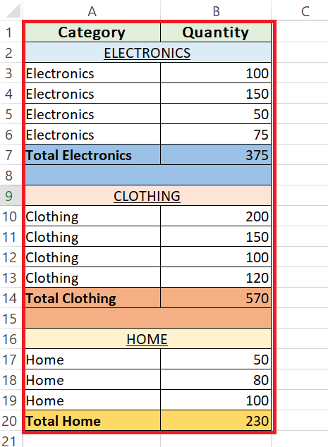
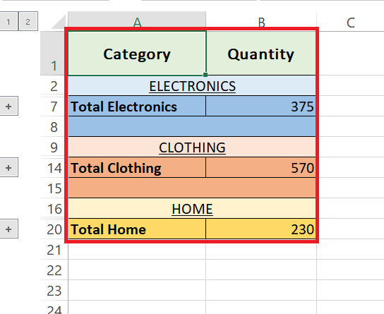
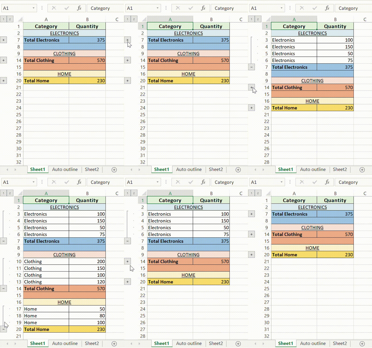
Smoothened dataset with the help of Grouping of rows.

 

Mastering the Basics of Row Grouping

How to Manually Group Rows in Excel

To manually group rows in Excel, you’ll want to start by selecting the rows you wish to group. This can be done by clicking on the row numbers on the side of your spreadsheet. If your rows are adjacent, simply click the first row, hold down the ‘Shift’ key, and click the last row in the series. For non-adjacent rows, use the ‘Ctrl’ key instead to select them individually.

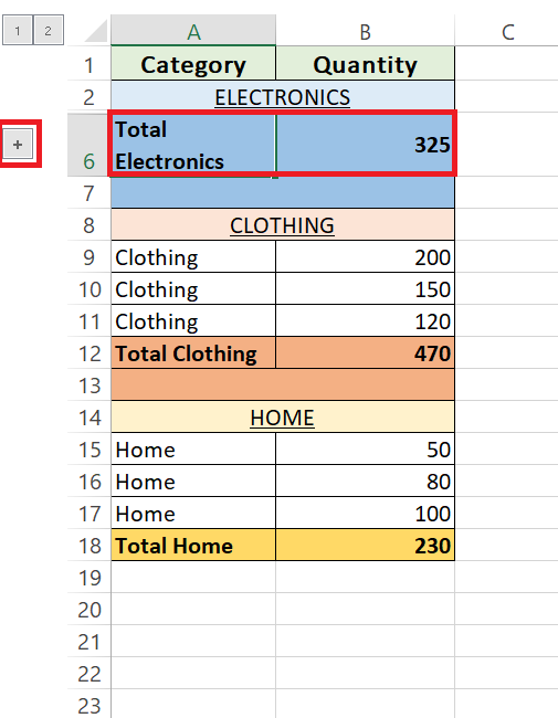
Once the desired rows are selected, head to the ‘Data’ tab on the ribbon at the top. Look for the ‘Group’ button, and click it to group the chosen rows. A small icon will now appear next to your groups, which enables you to expand or collapse your grouped data with a simple click, thus toggling between a detailed view and a summary view.

It’s a simple yet powerful step that brings immediate structure to your data. And if you just follow these instructions, give yourself a round of applause – you’ve leveled up your Excel skills!

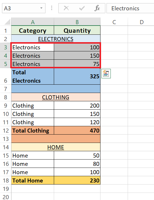
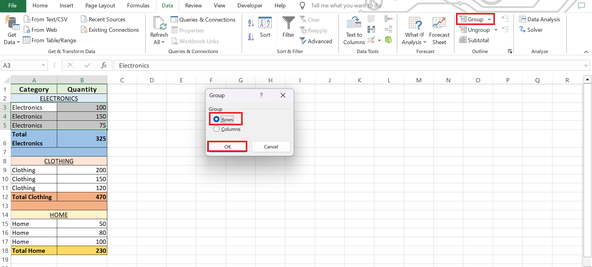
STEP 1: Select the rows you want to group.

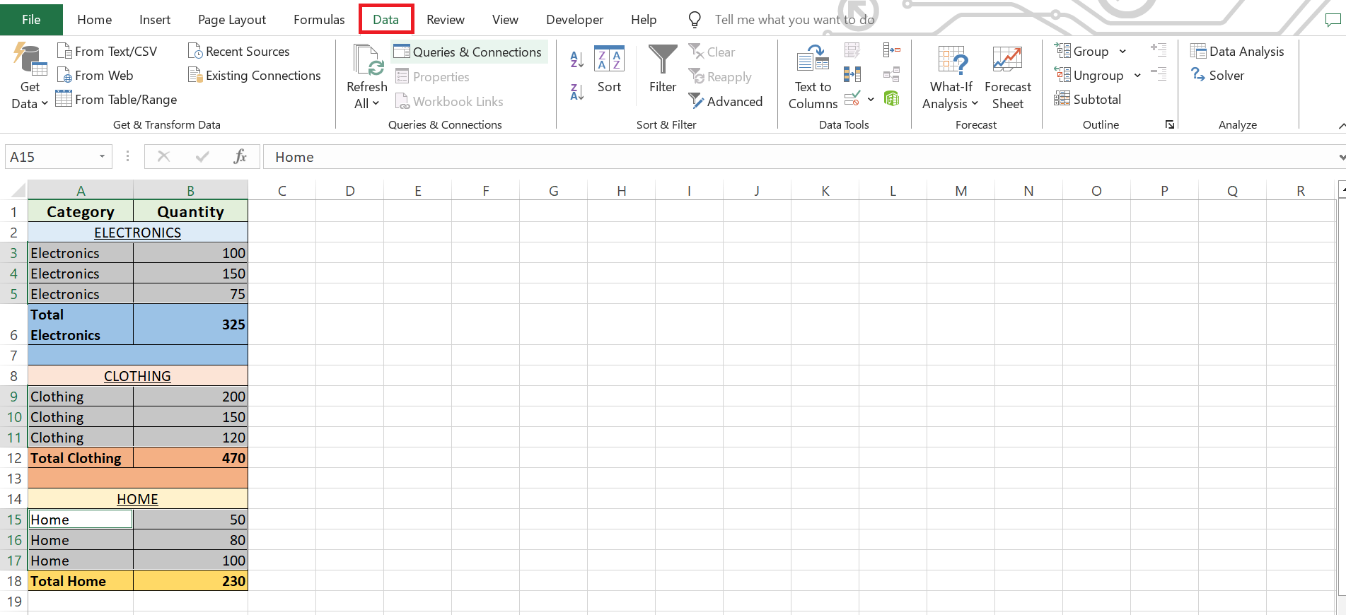
STEP 2: Navigate to the ‘Data’ tab on the ribbon.

STEP 3: Click the ‘Group’ button in the ‘Outline’ group. Select ‘Rows’ from the dialog box and click ‘OK’

RESULT: Excel will group the selected rows, and a small icon will appear next to the grouped rows for easy collapsing and expanding, providing a summarized or detailed view of your data.

 

Advanced Techniques for Clarity

Collapsing and Expanding Groups for Better Visibility

One of the most useful features of Excel grouping is the ability to hide and show the detailed rows for a particular group as well as to collapse or expand the entire outline to a certain level in a mouse click. This is particularly helpful for when you’re looking to streamline a large amount of data into a more digestible format. You have nested data or groups within groups, hierarchy is key, and Excel simplifies it for you.

To collapse a group, position yourself within the grouped rows and look for the ‘-‘ symbol in the margins or header. Clicking this symbol consolidates your data, giving you a cleaner, high-level view. But wait, you need details? No problem—just look and click on the ‘+’ sign to expand and bring back all the rows into view.

This flexibility to toggle between a condensed and expanded format not only aids in better visualization but also enables others who may be interpreting your spreadsheet to follow along without getting lost in an ocean of data.

 

Calculating Subtotals Within Grouped Rows

When you’ve got grouped rows, calculating subtotals is a breeze, and it makes your data so much more digestible. Imagine being able to swiftly summarize different segments of your information without manually crafting formulas for each section.

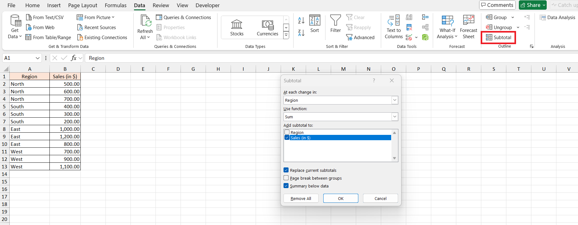
To sprinkle a little magic on your data, you’ll want to use the Subtotal command found under the ‘Data’ tab in the ‘Outline’ group. After choosing the range you’d like to subtotal, this nifty tool will ask you where you want to add the subtotal and which function to use—be it summing, averaging, or counting your data, among others.

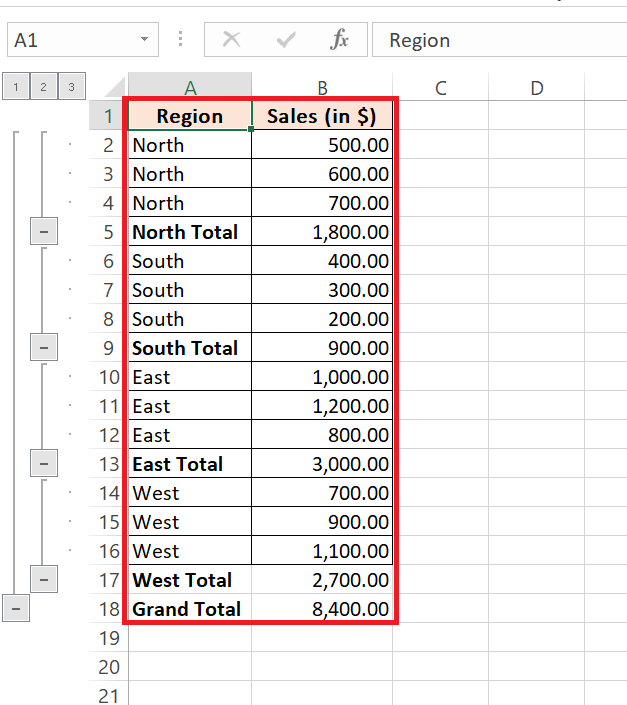
What’s more, Excel’s Subtotal function does a couple of neat things at once. It not only inserts those handy summary rows but also creates an outline with the ability to collapse and expand rows. This keeps your work streamlined and provides a grant total that updates dynamically as your data changes.

To insert subtotals:

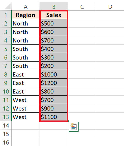
STEP 1: Select the range you want to subtotal.

STEP 2: Go to the ‘Data’ tab, find the ‘Outline’ group, and click on ‘Subtotal’.

STEP 3: In the Subtotal dialog box, at each change in (e.g., Sales), the function (e.g., Sum), and which column to add the subtotal to (e.g., Sales). Click OK.

This will automatically insert subtotals for each region and create an outline that allows collapsing and expanding rows.

 

Tips and Tricks for Efficient Data Management

Keyboard Shortcuts to Speed Up Your Workflow

Who doesn’t love a good shortcut? They’re like your Excel productivity cheat codes. Keyboard shortcuts are a fantastic way to navigate through your spreadsheets more quickly and efficiently, minimizing use of the mouse, which can really slow you down.

Speed Up Collapsing and Expanding

• Alt + Shift + – : Collapse grouped rows.
• Alt + Shift + = : Expand grouped rows.
• Ctrl + 8 : Show or hide the outline symbols.

Navigate with Ease

• Ctrl + A : Select the full sheet.
• Alt + A + H : Collapse all groups.
• Alt + A + J : Expand all groups.

Macabacus add-ins go even further, offering over 100 custom shortcuts, including collapsing and expanding grouped rows and columns with simple key combinations. If you frequently need Excel-to-PowerPoint linking or additional productivity tools, a Macabacus free trial could be worth a shot.

Remember, mastering these shortcuts won’t happen overnight, but with consistent practice, you’ll begin to cruise through your spreadsheets with impressively swift keystrokes. And the best part? More time to relax with that cup of coffee!

Applying Default Styles for Consistent Summary Rows

Excel’s default styles for summary rows—RowLevel_1 (bold) and RowLevel_2 (italic)—not only add a visual hierarchy but also ensure consistency across your spreadsheets, making them easier for everyone to follow.

Applying these styles can be as simple as selecting your summary rows and choosing the desired style from the ‘Styles’ group under the ‘Home’ tab. But to go one step further, you can make Excel automatically apply these styles when you create an outline.

How to set automatic styling:

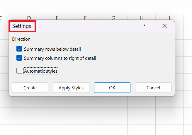
STEP 1: Go to the ‘Data’ tab and select ‘Outline’. Click the dialog box launcher.

STEP 2: ‘Settings’ dialog box is displayed.

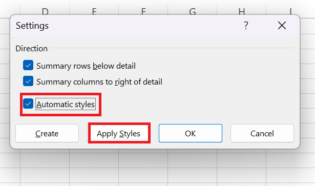
STEP 3: Select ‘Automatic styles’ and voilà, Excel now styles summary rows for you!

To apply styles to an existing outline, go through a similar path: ‘Data’ > ‘Outline’; ensure ‘Automatic styles’ is checked and hit ‘Apply Styles’. Simple as that!

Your spreadsheets will instantly look more polished with bold and italic stylings demarcating different levels of data groups. This is a small touch that can make a big difference to how quickly readers can grasp the structure and key points of your dataset.

 

FAQs on Grouping Rows in Excel

Can You Group Rows Based on Cell Values?

Yes, you can group rows in Excel based on specific cell values by using the Sort & Filter feature first to organize your data and then manually grouping the rows, or by creating a PivotTable, which automatically groups data according to the values you specify. The PivotTable is particularly powerful for this kind of task as it also allows for easy manipulation and summarization of the grouped data.

How Do You Handle Grouping in Large Datasets?

Handling grouping in large datasets requires a balance between detail and manageability. Start by determining meaningful categories for grouping that will simplify analysis without losing critical information. Use Excel’s ‘Subtotal’ feature for an initial layer of automatic grouping based on specific criteria, which is ideal for large datasets. Then, apply manual grouping as necessary for deeper analysis. Remember to expand all groups before applying filters or sorts to ensure no data is inaccurately excluded.

What is the shortcut for grouping rows in Excel?

The keyboard shortcut to group rows in Excel is Shift + Alt + Right Arrow. This convenient shortcut allows you to quickly group selected rows without having to navigate through the toolbar menus, significantly speeding up your workflow.

How do I group consecutive rows in Excel?

To group consecutive rows in Excel, click on the number to the left of the first row you want to group, then while holding down the Shift key, click on the number of the last row in the sequence to select the range. Next, go to the Data tab, and click on ‘Group.’ Now, your consecutive rows are neatly grouped together!

How does ungrouping work in Excel?

Ungrouping in Excel is a straightforward process that reverses the grouping action, allowing you to view all of your data again. To ungroup rows, you’ll first need to select the grouped rows that you wish to ungroup. You can do this by clicking on the row numbers on the left of your spreadsheet.

Once selected, head over to the ‘Data’ tab on the Excel ribbon. In the ‘Outline’ group, click on ‘Ungroup,’ then select ‘Ungroup’ again from the options provided. Excel will then remove the group, and the rows will no longer be collapsible—returning the spreadsheet to its original, fully expanded state.

Remember, if you have nested groups and only want to remove a specific level of grouping, you’ll need to select the appropriate rows before ungrouping. Ungrouping does not delete any data; it simply removes the hierarchy structure you’ve previously applied.