How to Hide Rows in Excel

When working with large spreadsheets in Excel, it can be helpful to hide certain rows to keep your workspace organized and focused. Whether you’re looking to declutter your view or temporarily hide data you don’t need, Excel offers several easy methods to accomplish this. In this article, I’ll walk you through how to hide rows in Excel step by step, so you can streamline your workflow and manage your data more efficiently.

Key Takeaways:

• Hiding rows in Excel helps keep your workspace organized and focused.
• You can hide rows using right-click, ribbon options, or keyboard shortcuts.
• Hiding unused rows can create a more focused work area in large spreadsheets.
• Advanced techniques like VBA scripts offer greater control over row visibility.
• Troubleshooting tips are essential for resolving issues like rows that won’t unhide.

 

Introduction

The Art of Organizing Excel Sheets

When we talk about Excel, we often envision spreadsheets cluttered with data – the bigger the dataset, the more overwhelming it can seem. However, with a strategic approach to organizing Excel sheets, it’s possible to transform them into polished reports ready for presentations or intuitive dashboards for daily use.

Organizing involves not just sorting and coloring but also skillfully managing which data remains visible. That’s where the ability to hide and unhide rows and columns in Excel comes in handy.

Understanding the Excel Workspace

To effectively use Excel, it’s crucial to understand the workspace it provides. At its core, the Excel workspace consists of an infinite number of rows and columns forming cells where data is entered. The intersection of a row and a column is where we input, analyze, and manipulate data. Understanding the grid-like structure aids in sorting, formatting, and, indeed, hiding or unhiding rows and columns as necessary.

The workspace is scalable; one can zoom in and out for better visibility or to work comfortably with large datasets. It also includes toolbars and ribbons that house an array of functionalities tailored for different tasks, including data management, which encompasses our ability to hide rows and columns as needed.

 

How to Hide Rows in Excel

Method 1: Right-click to Hide

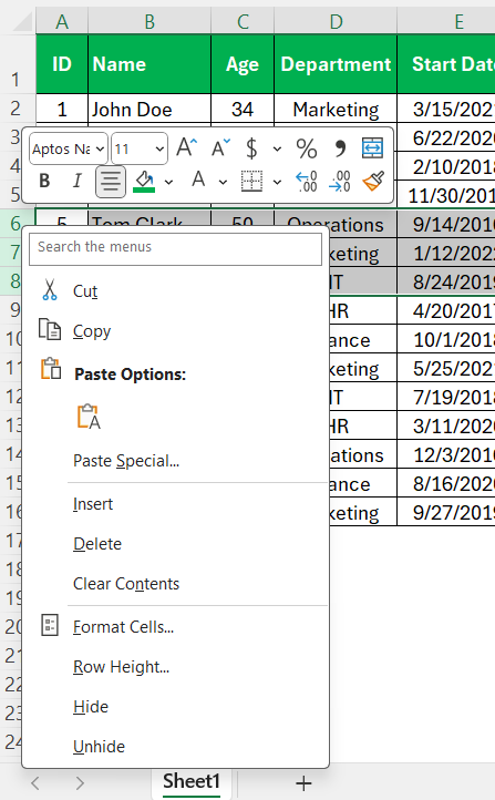
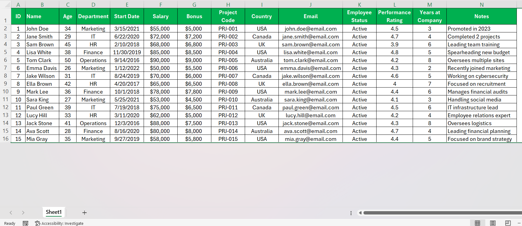
The first method I utilize to quickly hide rows or columns relies on the classic right-click context menu in Excel. Perform the following steps:

STEP 1: By selecting the row headers or column letters for the rows and columns I want to conceal, a right-click opens up a menu with various options.

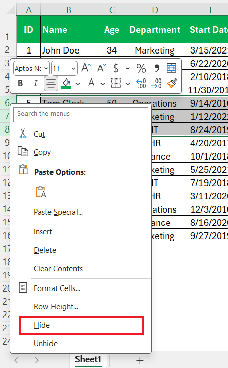
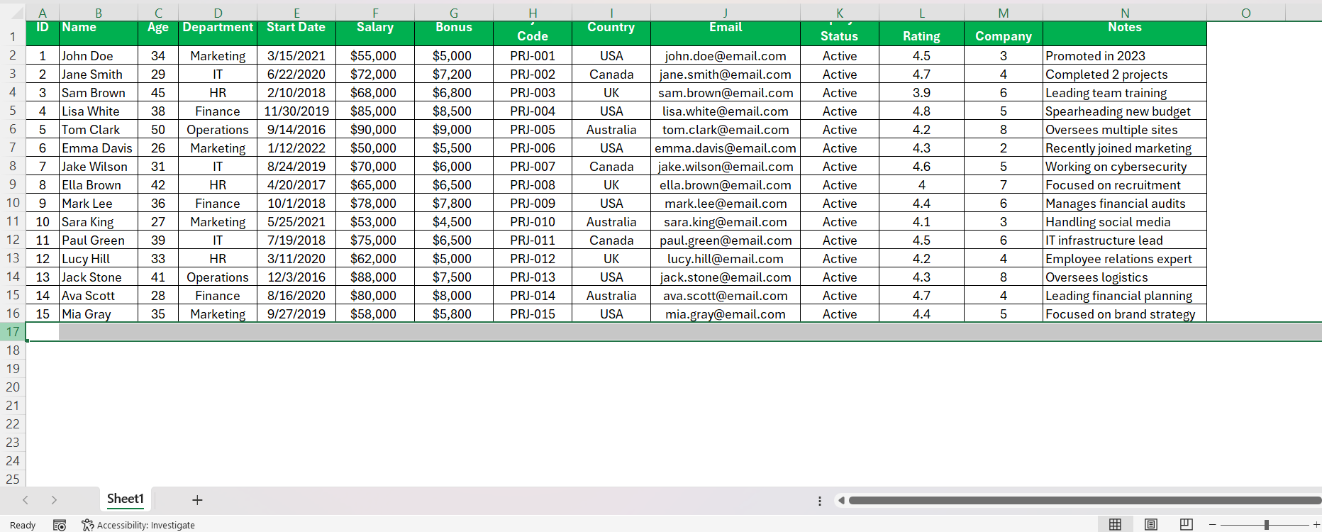
STEP 2: Among those, I click ‘Hide’, and just like that, the selected rows or columns disappear from view, leaving only a subtle indicator of their existence.

It’s like they’ve taken a step back from the spotlight, still there but allowing other data to take center stage.

This method is convenient, straightforward, and doesn’t require memorizing shortcuts or navigating ribbons – perfect for users who prefer mouse navigation over keyboard commands.

Method 2: Ribbon Customization and Shortcuts

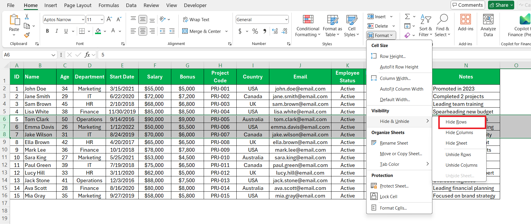
For the second method, I optimize the power of the Home tab in Excel’s ribbon. Follow these steps:

STEP 1: The process begins by selecting the rows I want to hide.

STEP 2: Here, under the Home tab lies the ‘Cells’ group, where the ‘Format’ button resides.

STEP 3: After clicking on ‘Format,’ I can weave my way to ‘Hide & Unhide’ and finalize my action by selecting ‘Hide Rows.’

Method 3: Using the Keyboard shortcut

Moreover, if I prefer keyboard efficiency, there’s a shortcut: Ctrl + 9. With one swift combo, the selected rows are neatly tucked away.

 

Going Beyond Basic Row Hiding

Hide Unused Rows for Focused Work Areas

Focusing on pertinent data is paramount, especially when dealing with extensive spreadsheets. To create a concentrated work area, I hide unused rows with ease. Let’s check the process:

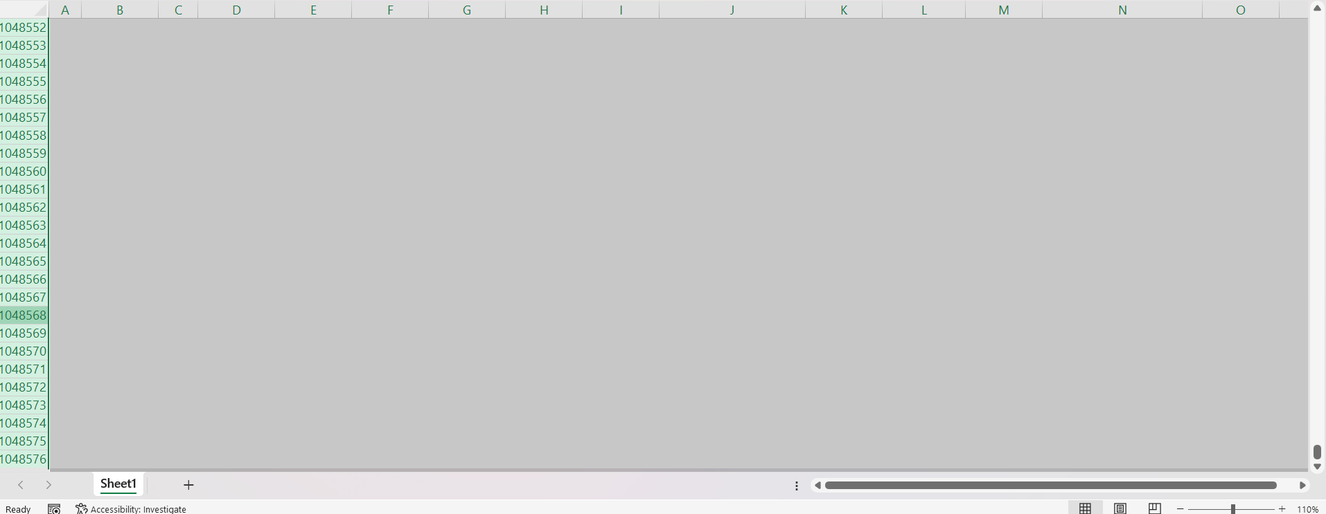
STEP 1: I select the row immediately following my dataset’s last row.

STEP 2: Then, holding Ctrl + Shift, I press the Down arrow to extend the selection to the spreadsheet’s bottom.

STEP 3: With a simple press of Ctrl + 9, those superfluous rows vanish, decluttering my workspace and allowing the necessary data to shine.

It’s akin to removing a curtain that’s hiding part of the stage; what’s left is just the scene I need to see.

Advanced Techniques: Grouping and Custom VBA

When I delve into advanced Excel techniques, custom VBA scripts stand out for managing the visibility of rows and columns.

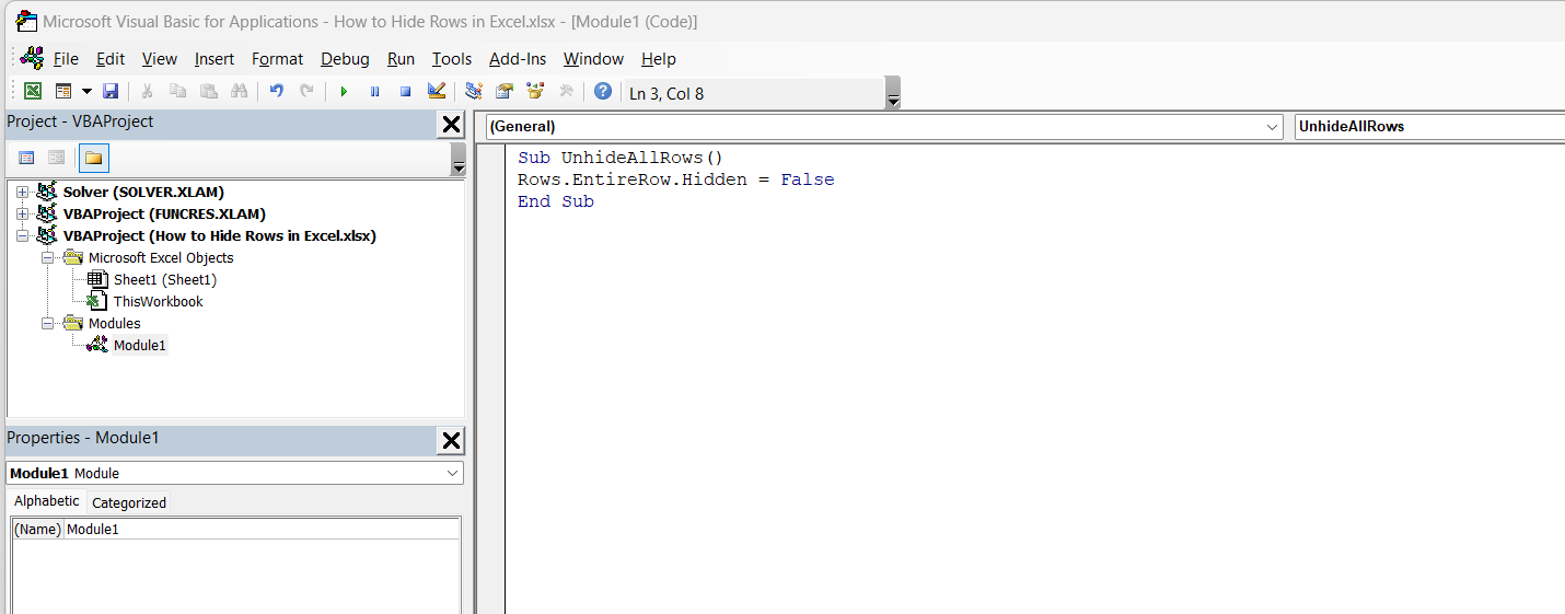
For even more control, I craft custom VBA scripts. By pressing ‘ALT + F11’, I dive into the realm of Excel’s VBA editor. A simple script like the following can unhide rows with a flourish:

After saving this macro in a ‘Macro-Enabled Workbook’, running it with ‘Alt + F8’ resurrects all the hidden rows, like magic. Customization is key here; scripts can be tailored to specific needs, such as revealing rows based on certain criteria, adding immense value when working with complex data sets.

 

Troubleshooting Common Issues

Solutions for Cannot Unhide Rows Problem

There are times when we encounter the puzzling scenario where rows just won’t unhide, no matter what we seem to do. In such situations, I advise checking for several common issues that might be preventing the unhide action.

The first thing I do is ensure that I’m selecting the rows both above and below the hidden ones, as failing to do this is a common oversight. If this doesn’t work, I look for any filters or freeze panes that might be interfering and remove them if necessary. Should the issue persist, it may be due to the row height being set to a very minimal value; in this case, I select the hidden row lines and manually adjust the row height.

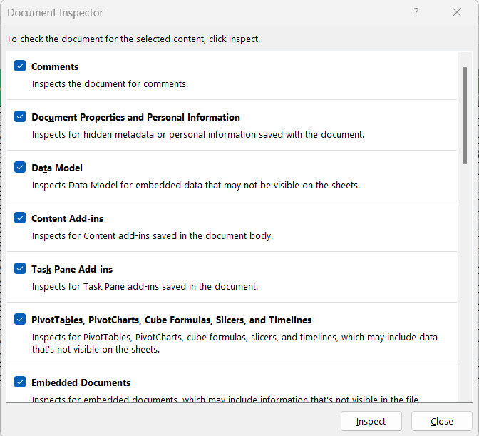
On occasion, the workbook might be shared or protected, which can restrict certain actions. If possible, I temporarily remove protection to perform maintenance on the sheet. Finally, if all else fails, turning to the ‘Inspect Document’ feature to remove any potentially corrupted hidden row states can be a lifesaver.

Tackling Filtered Rows and Protected Sheets

Handling filtered rows and protected sheets can be tricky. Excel’s filter feature lets us hide rows based on certain criteria without altering the row visibility settings directly.

If my goal is to work on filtered datasets or unhiding rows that have been filtered, I first check for the filter icon in the data headings. To clear all filters and reveal rows, I click ‘Sort & Filter’ on the Home ribbon and select ‘Clear’.

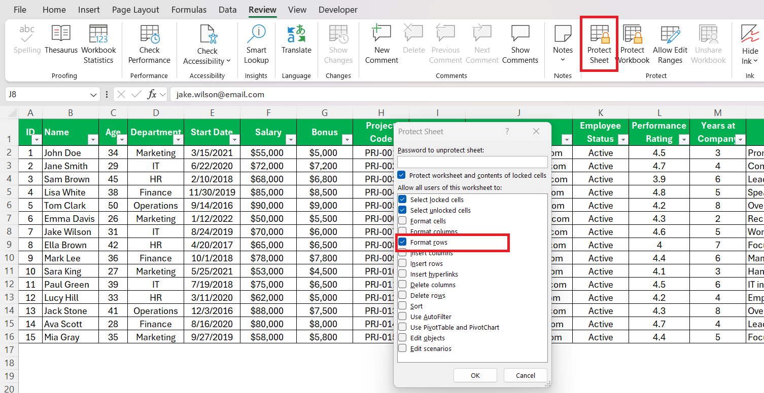
Working with protected sheets is another scenario. To ensure the data integrity isn’t jeopardized, protecting sheets can be necessary, but this also prevents modifications like hiding or unhiding rows. If I have the required permissions, I take these steps:

I click on the ‘Protect Sheet’ button on the Review tab, ensure that the ‘Format rows’ option is checked, and then confirm with ‘OK’.

This way, I can modify row visibility while keeping the sheet secured.

It’s crucial to comprehend these exceptions to seamlessly navigate Excel’s sophisticated organizational options.

 

Tips and Tricks for Efficiency

Keyboard Shortcuts to Streamline Your Workflow

Keyboard shortcuts are the secret sauce that speeds up my workflow in Excel significantly. For instance, hiding selected rows with Ctrl + 9 or columns with Ctrl + 0 feels near instantaneous compared to traditional point-and-click methods. Unhiding rows with Ctrl + Shift + 9, and columns with Ctrl + Shift + 0, brings them back just as quickly.

I frequently use ‘Alt + E, S, V’ to paste special, and Ctrl + Arrow keys to jump to the edge of data regions. ‘Alt + A, J’ and ‘Alt + A, H’ become natural when I work with grouping, allowing me to expand or collapse grouped rows or columns with ease.

These are just a few keystrokes elevating my Excel navigation from functional to lightning-fast. Over time, muscle memory kicks in, and these shortcuts become an intuitive aspect of my data management.

FAQs

How can I quickly unhide all hidden rows in Excel?

To swiftly unhide all hidden rows in Excel, I can click the Select All button or use Ctrl + A to select the entire sheet. If the first press of Ctrl + A selects only the current range, pressing it again selects the whole sheet. With the entire sheet selected, I can either use the keyboard shortcut Ctrl + Shift + 9, right-click and choose ‘Unhide’, or go to the Home tab, click ‘Format’, and then ‘Unhide Rows’. Any of these methods reveals all previously hidden rows efficiently.

What should I do if I cannot see the “+” indicator for expanding hidden rows?

If the “+” indicator for expanding hidden rows isn’t visible, it’s likely that the rows aren’t grouped but just hidden. To reveal them, select the rows immediately above and below the hidden rows, right-click on the row numbers, and choose ‘Unhide’. If it’s a case of missing grouping indicators due to toggled settings, I can re-enable them by going to Excel Options, Advanced, and checking “Show outline symbols if an outline is applied”.

How do I hide multiple rows in Excel?

To hide multiple rows in Excel, I click and drag across the row headings to highlight the rows I want to conceal. Alternatively, I can click on the first row, hold down the Shift key, and click on the last row of my selection range. Then, I can either right-click and choose ‘Hide’ or hit Ctrl + 9 to hide them all at once. It’s a straightforward process that keeps my workbook looking uncluttered and focused on the most pertinent information.

What is the shortcut for hide row in Excel?

The shortcut to hide a row in Excel is Ctrl + 9. After selecting the row or rows that I want to hide, pressing these keys instantly conceals them from view, without having to navigate through any menus or use the mouse – a real time-saver when I’m working through data and need to streamline my view quickly.

How do you unhide all columns in Excel?

To unhide all columns in Excel, I first select the entire sheet by clicking the Select All button or by pressing Ctrl + A twice. Then I use the keyboard shortcut Ctrl + Shift + 0, which quickly reveals all the previously hidden columns. Alternatively, I can go to the Home tab, click on ‘Format’, under the ‘Visibility’ section, choose ‘Hide & Unhide’, and then select ‘Unhide Columns’. It’s a simple process to ensure that no data remains hidden from view.