How to Highlight Unique Values in Excel

Normally when we have dirty data, we tend to get a lot of duplicates. If you want to spot the ones with unique values and highlight them, it is very easy to do in Excel for your data cleanup!

Key Takeaways

• Conditional Formatting Makes It Easy – Excel’s Conditional Formatting tool allows you to highlight unique values without using complex formulas.

• Built-in Rule for Unique Values – You can use Home → Conditional Formatting → Highlight Cells Rules → Duplicate Values and select “Unique” to highlight distinct values.

• Use COUNTIF for More Control – The COUNTIF function (=COUNTIF(A:A, A1)=1) can be used in Conditional Formatting for more precise highlighting of unique values.

• Apply Formatting Dynamically – When data changes, Excel updates the highlights automatically, ensuring real-time visibility of unique values.

• Works in Large Datasets Too – Even in large spreadsheets, highlighting unique values using Conditional Formatting is efficient and doesn’t slow down performance.

Our Data Setup

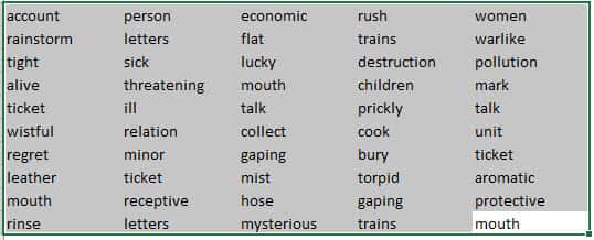
Here is our sample list of words, there are some duplicates and we only want to highlight the unique ones:

STEP 1: Select your list of words / data:

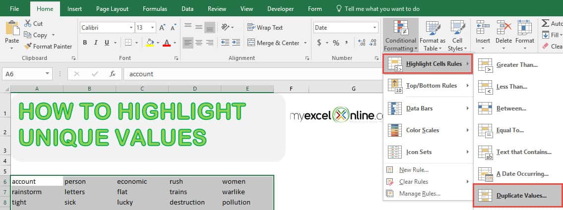
STEP 2: Go to Home > Conditional Formatting > Highlight Cells Rules > Duplicate Values

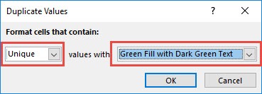
STEP 3: Make sure to select Unique so that the unique values will only be highlighted. You can select the formatting that you want. For our example, we selected Green Fill with Dark Green Text. 

Click OK.

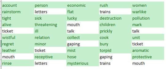
Excel is smart enough to highlight all of the unique values for you!

Frequently Asked Questions

How do I highlight unique values in Excel without a formula?
Use Conditional Formatting → Highlight Cells Rules → Duplicate Values, then select Unique to highlight distinct entries.

Can I use a formula to highlight unique values?
Yes! Apply Conditional Formatting using the formula =COUNTIF(A:A, A1)=1 to highlight only the unique values in column A.

Will the highlighting update if my data changes?
Yes! Conditional Formatting updates automatically when you add or remove values, ensuring accurate highlighting.

How do I highlight unique values across multiple columns?
Use COUNTIFS instead of COUNTIF, such as =COUNTIFS(A:A, A1, B:B, B1)=1, to check uniqueness across multiple columns.

Can I remove unique values instead of highlighting them?
Yes! You can use the Advanced Filter under the Data tab to filter out unique values or remove them manually.

Bryan

Bryan Hong is an IT Software Developer for more than 10 years and has the following certifications: Microsoft Certified Professional Developer (MCPD): Web Developer, Microsoft Certified Technology Specialist (MCTS): Windows Applications, Microsoft Certified Systems Engineer (MCSE) and Microsoft Certified Systems Administrator (MCSA).

He is also an Amazon #1 bestselling author of 4 Microsoft Excel books and a teacher of Microsoft Excel & Office at the MyExecelOnline Academy Online Course.