How to Lock Cells in Excel Worksheets

Locking cells in Excel is a vital technique I use to protect my data from unintended changes and ensure the integrity of my spreadsheets. By selectively locking cells, I can allow users to view and interact with certain parts of my worksheet while safeguarding critical data from edits. In this guide, I’ll walk you through the steps on how to lock cells effectively, ensuring your data remains secure and unaltered.

Key Takeaways:

• Introduction to Worksheet Protection: Locking cells is essential for protecting data integrity and preventing accidental or unauthorized changes in Excel.
• Importance of Locking Cells: This practice safeguards critical information, such as formulas and sensitive data, from being altered inadvertently.
• Common Scenarios for Using Cell Protection: Cell protection is useful for preserving the accuracy of budget spreadsheets, financial models, and educational templates, among other applications.
• Essential Steps to Safeguard Your Data: To lock specific cells, unlock all cells first, then select and lock the desired cells before protecting the sheet to enforce the lock.
• Streamlining the Locking Process: Adding the ‘Lock Cell’ option to the Quick Access Toolbar and mastering keyboard shortcuts can speed up and simplify the cell protection process.

 

Introduction to Worksheet Protection in Excel

The Importance of Locking Cells

Locking cells in Excel plays a crucial role in maintaining the integrity of a worksheet’s data, especially in a collaborative environment. I consider it an imperative measure to ensure that important calculations are not altered inadvertently.

When we lock cells, we’re putting up a safeguard against accidental or unauthorized changes, which could otherwise lead to errors, misinformation, or even data breaches. Essentially, it’s all about retaining control over a spreadsheet’s content and preserving its reliability.

Common Scenarios for Using Cell Protection

We often encounter situations where cell protection in Excel is not just helpful, but necessary. For instance, when creating a budget spreadsheet, it’s commonly preferred to lock cells containing categories or formulas calculating totals to prevent alterations that could skew the budget.

In a business setting, protecting sensitive data such as pricing models, financial projections, or proprietary formulas is crucial to safeguard the company’s interests. Educational institutions may use cell protection to create standardized tests or assignment templates, where students can input answers without disrupting the structure or scoring mechanisms. These scenarios underscore how cell protection tailors Excel to suit its versatile roles across different sectors and use cases.

 

Essential Steps to Safeguard Your Data

Step-by-Step Approach to Lock Individual Cells

To lock individual cells in Excel, one needs to navigate the typically unlocked terrain of a fresh worksheet, selectively preserving the sanctity of specific cells. Here are the footsteps I follow to achieve this:

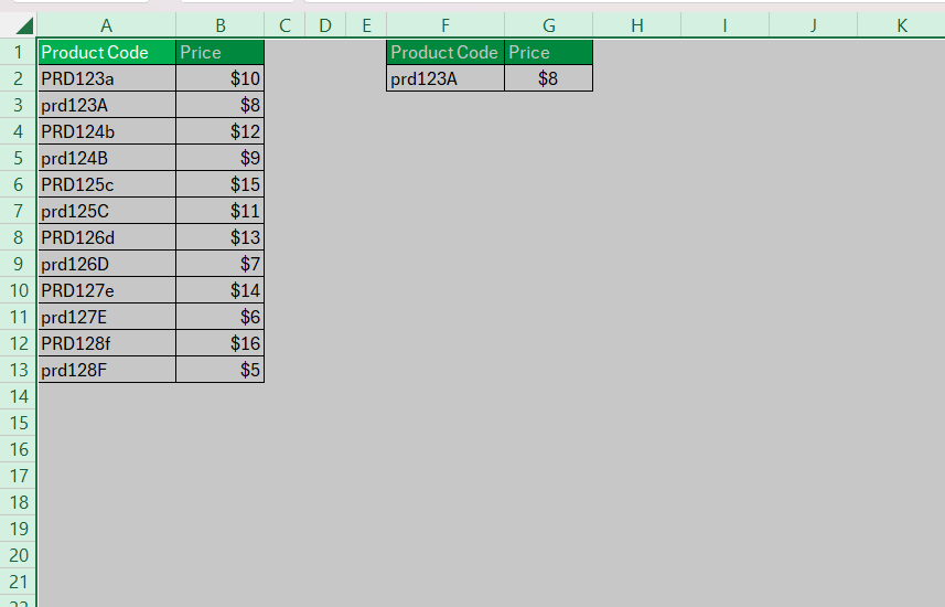
STEP 1: Begin with a grand selection of all cells by pressing CTRL + A.

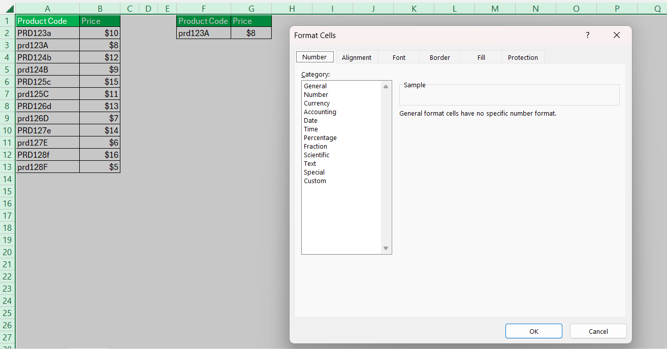
STEP 2: Offer a right-click on any cell, or if you’re partial to keyboard strokes, CTRL + 1 will summon the Format Cells dialogue.

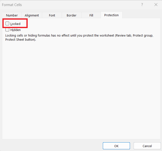
STEP 3: Gracefully uncheck the Locked option under the Protection tab and click OK.

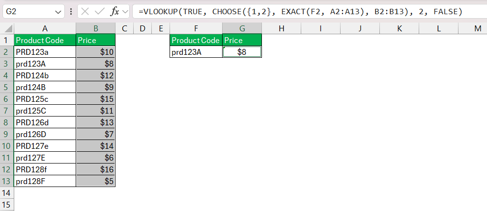
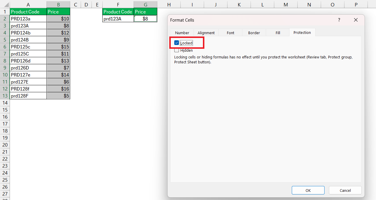
STEP 4: Now, let’s say range B2:B13 and G2 are the chosen ones. Select them as the guardians of your data.

STEP 5: A right-click once more, CTRL + 1 for the Format Cells, and this time, under Protection, bestow upon them the check of ‘Locked’.

Remember, until the worksheet is protected, these cells are as vulnerable as any other.

STEP 6: Finally, protect the sheet under the Review tab or using the ALT + R + P incantation, and voila, A1 and A2 are the untouchables amidst a field of openness.

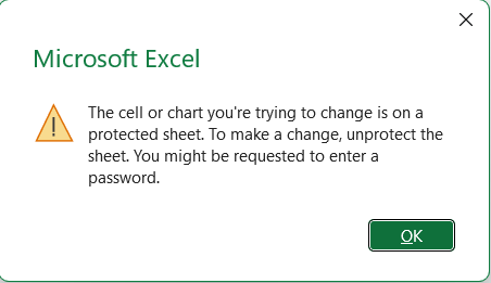
When we try to edit those locked cells, we will see the error message as shown below –

How to Secure Formula Cells Without Hassle

Securing formula cells to prevent tampering is a breeze once I walk you through the seamless steps to protect the lifeblood of your spreadsheet – the formulas. Here’s what I do to keep those valuable cells under a vigilant watch:

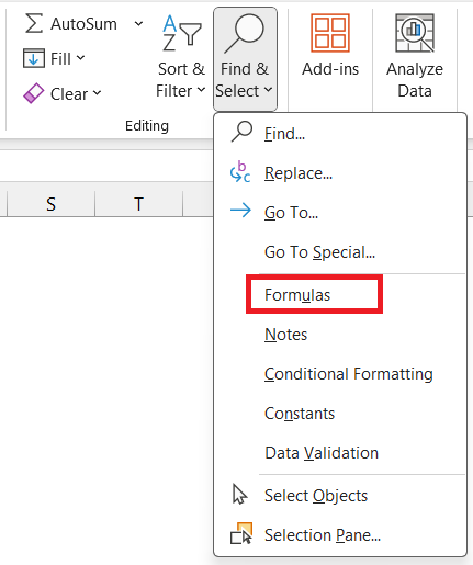
STEP 1: After unlocking all cells as detailed previously, navigate to the Home tab, identify the Editing group, and click on the dependable ‘Find & Select’.

STEP 2: Choose ‘Formulas’ from the options.

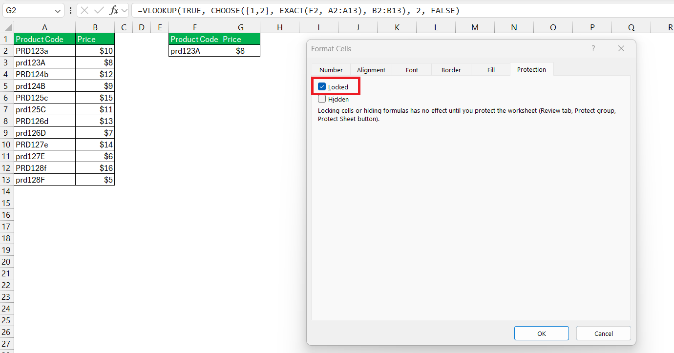
STEP 3: With all formula-bearing cells now selected, a quick CTRL + 1 beckons the Format Cells box where the Locked checkbox waits eagerly for a tick.

And for those who seek the shadows, the Hidden checkbox can make even the formula itself disappear from the formula bar upon cell selection – a veil of secrecy.

Setting the final seal on my work, I return to protect the sheet, which entails choosing to ‘Protect Sheet’ and, optionally, adding a password to wield that key to the kingdom.

Now, try editing a cell that houses a formula – it rebuffs any advances with unwavering resolve. Only through unprotecting the sheet, which requires the password, can the formulas be altered, preserving my data’s purity and my peace of mind.

Unlocking Specific Ranges for Collaborative Work

When it’s necessary to navigate the tightrope of collaborative work, where access must be selectively granted, unlocking specific ranges of a protected worksheet allows for such focused collaboration. I’ve found the following steps enable this delicate balance of protection and teamwork:

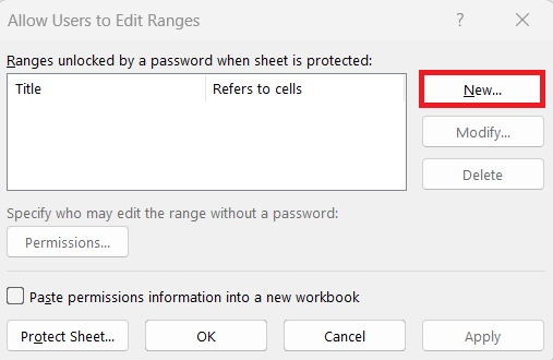
STEP 1: With the worksheet initially protected, I switch to the Review tab where the ‘Allow Users to Edit Ranges’ command awaits my signal.

STEP 2: Upon selecting it, a dialog box presents itself, listing any existing ranges available for editing. To add new ones, I click ‘New’.

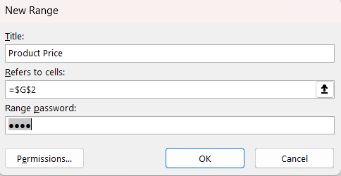
STEP 3: I define the range for my collaborators to access by typing in the cells’ reference or selecting the range directly in the worksheet.

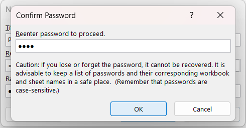
STEP 4: A prompt to enter a password appears, which, when set, restricts editing to those with the password or permission.

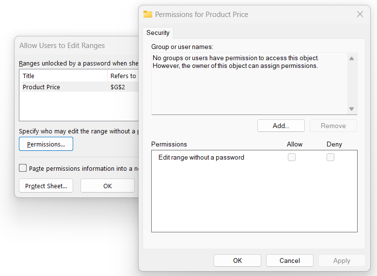
STEP 5: The final act is to specify permissions. I click ‘Permissions’, then ‘Add’, and enter the names of the users or groups I’m granting access to.

Excel and I come to an agreement on the user names, and upon my confirmation, the designated cells become available for those selected individuals.

It’s worth noting that even when cells are unlocked, the remainder of the worksheet remains protected, ensuring both collaboration and control.

 

Streamlining the Locking Process

Quick Access Tools for Frequent Protectors

For those of us who often find ourselves in the trenches, protecting cell after cell against the potential missteps of collaborators, Excel’s Quick Access Toolbar emerges as a beacon of efficiency. Here’s how I streamline my protective efforts:

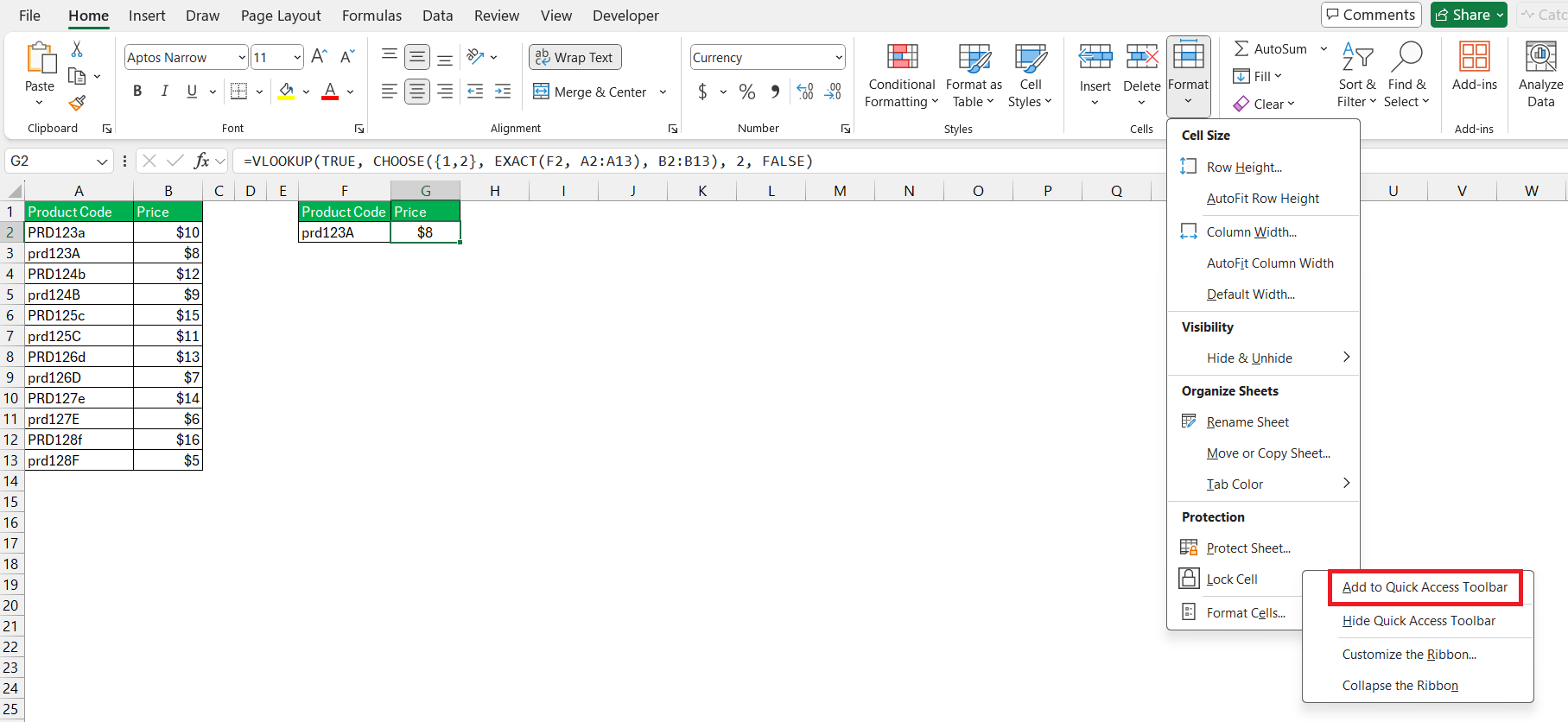
STEP 1: Go to the Home tab, seeking the Cell Format command with the fervor of a knight on a quest.

Upon sighting the option ‘Lock Cell’, I right-click it, drawing forth the context menu from which I deftly select ‘Add to Quick Access Toolbar’.

STEP 2: With this singular action, a new guardian icon takes its place among the toolbar’s elite, enabling me to lock or unlock cells with but a single click.

I’ve found that adding the Lock Cell option to the Quick Access Toolbar simplifies my task, allowing me to safeguard my data with the swiftness of an Excel virtuoso.

Keyboard Shortcuts to Expedite Protection Setup

To circumnavigate the labyrinth of mouse clicks, I invest my time in mastering keyboard shortcuts that expedite the protection setup in Excel. This mastery bestows upon me the ability to enact or lift a cell’s protective state with dexterity and speed:

• CTRL + A selects all cells, from whence I can tap CTRL + 1 to bring forth the Format Cells dialog and visit the Protection tab without delay.
• With this dialog open, hitting ALT + L toggles the Locked option, and ALT + H hides or reveals the formulas within the cells. A press on ‘Enter’ solidifies my choice.
• To protect the sheet swiftly, I press ALT + R, followed by P twice, inviting the Protect Sheet dialog into the limelight.
• If there’s a need for a password, I traverse the text box with TAB, where my keystrokes breathe life into a secret code that will guard my sheet.
• A final flourish of ‘Enter’ activates the sheet’s defenses, cloaking my data in protection as efficiently as a key turns in a lock.

By utilizing these shortcuts, I minimize my journey through menus and ribbons, reinforcing my data’s security with archival speed and precision.

 

FAQs

How do I lock specific cells in Excel?

To lock specific cells in Excel, first unlock all cells with CTRL + A and CTRL + 1 to open Format Cells, then uncheck ‘Locked’. Next, select the cells to lock, open Format Cells again, check ‘Locked’, and ‘OK’. Protect the sheet under Review to enforce.

How do you lock cells in Excel that you cannot edit?

You lock cells in Excel by right-clicking them, selecting Format Cells, checking ‘Locked’, and then protecting the sheet. Until you protect the sheet, the lock has no effect on cell editing.

How Do I Prevent Users from Editing Certain Cells?

Prevent users from editing certain cells by selecting them, opening Format Cells using CTRL + 1, checking ‘Locked’, and then applying sheet protection via the Review tab. Only unlocked cells remain editable after protection is enabled.

Can I Lock Cells and Still Allow for Sorting and Filtering?

Yes, I can lock cells and still allow sorting and filtering by setting the appropriate options in the Protect Sheet dialog. Check ‘Sort’ and ‘AutoFilter’ before finalizing sheet protection to keep these functionalities active.

How to lock cells when scrolling in Excel?

Lock cells when scrolling in Excel by using the Freeze Panes feature. Click on View, select Freeze Panes, and choose ‘Freeze Top Row’ or ‘Freeze First Column’. Multiple rows or columns can be frozen by selecting the cell below or to the right of them and choosing ‘Freeze Panes’.