6 Simple Ways to Merge Cells in Excel

Watch on YouTube and give it a thumbs up 👍

How to Use the Merge & Center button

A great way to customize the layout of your Excel worksheet is to use the Merge & Center feature in Excel.

It is a great way to create a label that spans several columns. This feature will retain the value in the upper-left cell but keep in mind that all data in the other merged cells will be deleted.

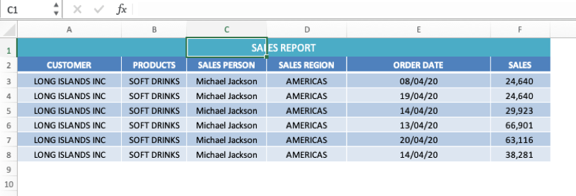
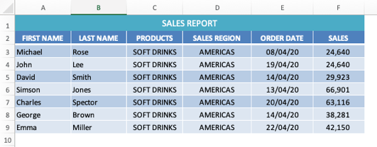
In the example below, you can see that the text “SALES REPORT” is located in a single cell in A1. Let us fix that!

Step 1: Select the cells A1:F1 that you want to merge.

Step 2: Go to Home > ‘Alignment’ group > Merge & Center button

Step 3: The currently selected cells will be merged, and their contents will be center aligned.

Notice that the reference for the 6 merged cells cell points at A1.

By following this step-by-step guide on How to Merge Cells in Excel you can create headers/titles for you report that will make it much easier to understand.

Other Merge & Center Options

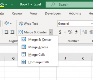
When you click on the drop-down arrow beside the Merge & Center button in the Alignment group, you will see it contains a drop-down list with additional options and each one produces a different result:

• Merge Across − When a multi-row range is selected, this command creates multiple merge cells in Excel — one for each row.
• Merge Cells − Merges the selected cells without applying the Center attribute.
• Unmerge Cells −This unmerges the merged cells in Excel and we explain in detail below.

 

Once you have learned how to merge cells in Excel, you should also know how to unmerge them. In order to Unmerge Cells in Excel

Step 1: Select the cells that you want to unmerge.

Step 2: Click the Merge & Center button or select the Unmerge Cells option from the drop-down menu.

Your data is now unmerged.

NB: Even though this is a fairly simple process to know how to merge cells in Excel, it is not highly recommended, and further below we explain the alternatives to merge cells in Excel.

If any data was lost when the original cells were merged, they will not be restored (unless your select CTRL + Z to undo the last action).

Here are a couple of shortfalls once cells have been merged:

• Excel Functions won’t work on merged cells
• Excel ‘Sort’ command will not work on ranges that contain the Excel merge cells.
• Single column can’t be selected if it contains any merged cells
• Excel Filters cannot be applied
• Dates cannot easily be copy-pasted elsewhere

Here is a video from Microsoft showing merging and unmerging cells in action.

Using Center Across Selection

To achieve the same result as Merge & Center without having the above restrictions, use the Center Across Selection feature. This would merge the cells across columns and still let you select each cell individually. Below we explain how to apply the Center Across Selection:

Step 1: Select the cells A1:F1 that you want to merge.

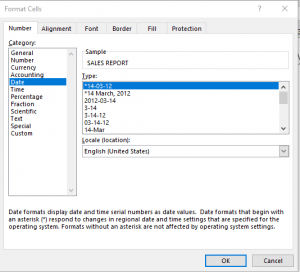
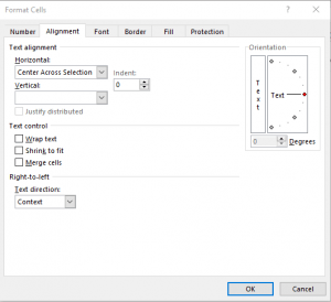
Step 2: Press Ctrl + 1 to bring up the Format Cells dialog box.

Step 3: Under the Alignment Tab, in the Horizontal drop-down box, select “Center Across Selection”

Step 4: Click OK.

The selected cells are now merged. You can see that even though the data is merged across cell A1: F1, you can still select and refer to each cell individually!

Using the CONCATENATE Function

If you use the above options to merge cells in Excel, it will keep the text at the leftmost cell (A1 in this case) and remove the text from all other cells. If you don’t want to lose the text from the merged cells in Excel, use the CONCATENATE Function (pre Excel 2019), the CONCAT Function (Excel 2019 & Office 365) or the ampersand “&” operator. The CONCATENATE function combines cells in Excel quickly.

There may be times when you are dumped with data in Excel and it is not formatted quite the way you want. Say, you have the First Name and Last Name in different columns and you want to merge them in a single column containing First & Last Name.

Now, if you use Merge & Center or Merge Across Selection, it will delete the text in the second column and only display the First Name as a merged cell. But this is not what you were looking for. Right?

Let me introduce you to the Concatenate Function and the ampersand “&” operator that will merge cells in Excel! This feature should definitely be bookmarked as it will come in handy when cleaning, transforming and analyzing data in Excel.

The Concatenate Function will merge multiple cells into a single cell and keep both values. You can merge or join more than two cells together whether it contains text, numbers, or both.

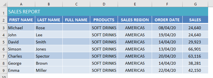
In the SALES REPORT below, you have the First Name in Column A and Last Name in Column B. For reporting and further analysis, you need them to be combined into one column, so it’s best to use the Concatenate function or the “&” Operator for this. It is perfect for when you want to merge cells or combine ‘FIRST NAMES’ with ‘LAST NAMES’ that are in separate columns and merging them into one cell.

Before I  get into how to merge cells in Excel, let’s talk about exactly what happens when you try to use Merge & Center here. If you select cells A3 and B3 and then press the “Merge & Center” button, you will see that you end up with an Excel merged cell with only the upper-left cell’s value i.e. the First Name.

To merge cells in Excel without losing any data, you should use the Concatenate Function in Excel. Follow the steps to know how to combine cells in Excel:

Step 1: Select Column C and press Ctrl + to add a new column. Name this column as “Full Name”.

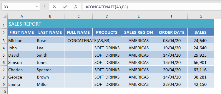
Step 2: Select Cell C3 and type the formula: =CONCATENATE(A3, B3). Press Enter

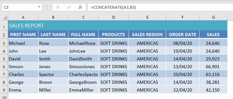
Step 3: Copy cell C3 and paste it in remaining cells or drag the fill handle to copy the formula to the other cells below.

This will merge cells in Excel without losing the data!  Below we show you how to make this merged cell look prettier by adding a space between the First & Last Names as well as a line break.

Adding a Space & Line Breaks while Merging Cells

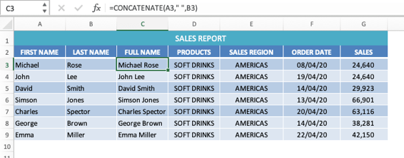
In the FULL NAME column above, you can see that there is no space or any character between the FIRST NAME and the LAST NAME. This mashed-together value of the FULL NAME isn’t a typographical mistake. It is important to understand how to combine cells in Excel including spaces.

To concatenate this information and include spaces, in the 2nd CONCATENATE function argument, you need to type in double quotation marks and put a space between these quotations i.e. ” “

The edited formula will be =CONCATENATE(A3,” “, B3).

You can replace the space with a dot, comma, or any other character. Simply, replace the space in this function with a character and make sure to enclose the character or text in double quotation marks. With the Concatenate function you also have the option to amend the combination later, whereas you don’t have any such option if you use Merge & Center.

You can also use the ampersand sign, &, to combine cells in Excel. The & operator works just like the CONCATENATE function where you can combine text, numbers, individual cells, etc. Both CONCATENATE and & produce the same results.

Let’s see how to merge cells in Excel using the & operator.

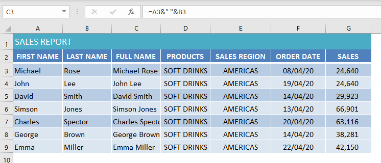
The following examples show the same SALES REPORT but this time I will use & operator to merge cells in Excel.

The formula to be used is = A3&” “&B3

You can see that the result is the same and you can use either the ampersand sign & or the CONCATENATE function, it just depends on what you are more comfortable with.

You can also add line breaks while merging cells by using the CHAR(10) function in Excel.

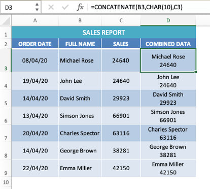
In the following example, the CHAR(10) function is used to add a line break between FULL NAME & SALES. You can use the formula: =CONCATENATE(B3, CHAR(10), C3).

Also, make sure you select the “Wrap Text” option under the Home Tab, otherwise the result will be displayed in the same line only.

You can see that the FULL NAME is displayed on the first line and the second line contains SALES, which is another cool way you can create Excel merged cells.

Bonus Approach – Flash Fill

Lastly, there is a BONUS approach to merge cells in Excel with – Flash Fill. It is probably the simplest way to combine cells in Excel and is available in Excel 2013 or later.

Flash Fill is a special tool that analyses the pattern from the existing cells and then automatically extracts the data to the pattern that you set. We can combine the FIRST NAME and LAST NAME from the previous example using Flash Fill.

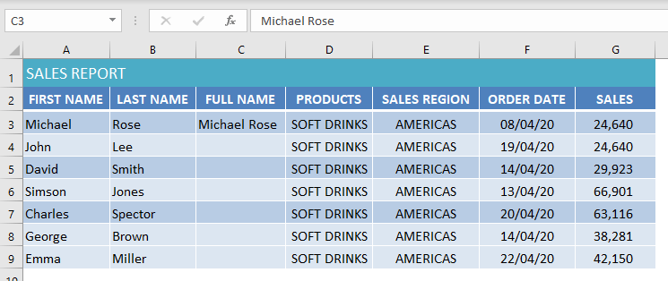
Step 1: You should establish a pattern by typing the FULL NAME in cell C2.

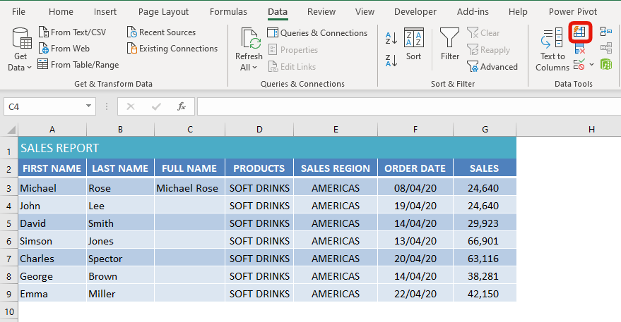
Step 2: Highlight the remaining cell and press the keyboard shortcut Ctrl + E or go to the ribbon menu and select: Data > Flash Fill

Step 3: Excel will sense the pattern you provided in C2, and will fill in the empty cells below, merging the FIRST NAME with the LAST NAME.

If the Flash Fill does not seem to be working for your data, make sure it is turned on.

To turn Flash Fill on, go to Tools > Options > Advanced > Editing Options > check the “Automatically Flash Fill” box.

Excel’s Flash Fill feature is a versatile tool that can be used to merge, split, or clean data. You need to type the first entry for Excel to sense the patterns and then Excel fills in the rest of the data based on the pattern you provided.

In Conclusion

So, the Merge & Center or Center Across Selection features in Excel makes data more visually presentable and highly organized. But it only keeps the contents of the top-left cell and deletes the rest.

This loss of data is a big disadvantage when you merge cells in Excel. To preserve your data in Excel, use the & operator, the CONCATENATE function, or Flash Fill to merges cells’ contents into one cell.

Make sure to download our FREE PDF on the 333 Excel keyboard Shortcuts here:

You can learn more on how to use Excel by viewing our FREE Excel webinar training on Formulas, Pivot Tables and Macros & VBA!

You can follow our YouTube channel to learn more about How To Merge Cells in Excel!

👉 Click Here To Join Our Excel Academy Online Course & Access 1,000+ Excel Tutorials On Formulas, Macros, VBA, Pivot Tables, Dashboards, Power BI, Power Query, Power Pivot, Charts, Microsoft Office Suite + MORE!