How to use Excel LET function

If you write long complex formulas in Excel, then the new LET function is a perfect match for you. It lets you define variables inside the formula and get calculation results. Excel LET function is useful when you use the same expression multiple times in a formula.

This function is available exclusively for Excel 365 subscribers.

Sign up to Office 365 to get access to all the cool updates and new functions that allow you to be more efficient in Excel.

In this article, you will be provided a detailed guide on the following:

• Introduction to Excel LET Function
• Syntax & Arguments
• LET with one name-value pair
• LET with five name-value pairs
• LET with Emojis
• LET using Name manager

Watch how to use the LET function in Excel on YouTube and give it a thumbs-up!

Download this Introduction to the Microsoft Excel LET Function Tutorial workbook so you can practice along with us:

 

Introduction to Excel LET function

You might have used Named Range in Excel while creating lengthy formulas and know how they make the formula easier to read. LET function is like an advanced version of named ranges.

It lets you assign names directly to the calculation. In this way, Excel calculates the value of the variables just once and uses it several times within the same formula.

The three benefits of using LET functions are:

• Improves formula readability – Assigning a user-friendly name to a range/variable and using it repeatedly in the calculation will make the formula cleaner, easier to read and understand.
• Improves performance – Excel LET function eliminates duplicate calculation. The expression is evaluated at the beginning of the formula and then reused multiple times without further calculation. This increases the speed and performance of the worksheet.
• Easier to update – If you need to change the value of the defined variable, you can easily change it at the beginning instead of updating the same expressions multiple times.

 

Syntax & Arguments

The formula breakdown of the Excel LET function is:

=LET (name1, value1, [name2], [value2], calculation)

where:

• name1 – the name of the first variable defined (it should be without spaces, period, or special characters);
• value1– the value that should be assigned to the first name (it can be text, number, cell reference, or formula);
• name2 – the name of the second variable (optional);
• value2– the value assigned to second variable (optional);
• calculation – the expression or formula that uses these defined variables.

For example:

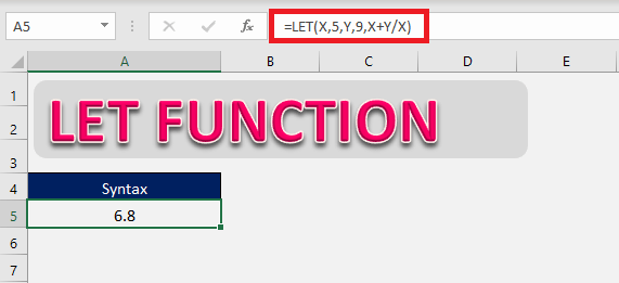
=LET(x, 5, y, 9, x+y/x)

Here, Excel will assign 5 to variable x, 9 to variable y, and then perform the calculation – 5+9/5. It will return the output as 6.8.

You can define numerous pairs of names and their values and insert a calculation that uses all of them. Excel can handle a total of 126 name-value pairs in this function.

Before you start using this incredible function, there are few things that you should note:

• LET function is not available in any of the older versions of Excel (2010, 2013, 2016, 2019). Only in Excel for Microsoft 365.
• The scope of defined names is limited to that formula only. You can reuse these assigned names multiple times within the formula but not anywhere else.
• There should be several name-value pairs but the last argument should be “calculation”.
• The name argument should start with a letter, an underscore (_), or a backslash (\). It cannot start with an “r” or “c” as they are reserved for the R1C1 style.
• The name argument should follow the same convention as the named range i.e. it should be without spaces, period, or special characters.

 

LET with one name-value pair

Let’s start with an easy example of one name-value pair to simply understand the working of the Excel LET function.

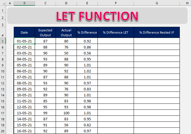
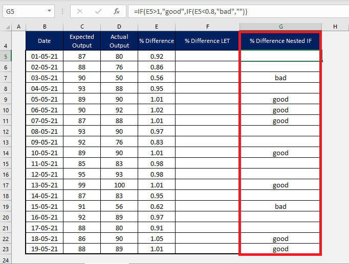
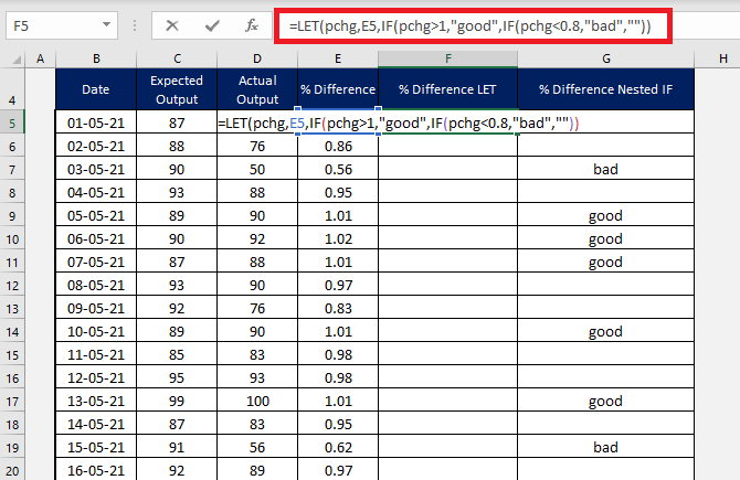
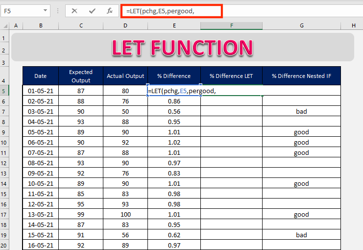
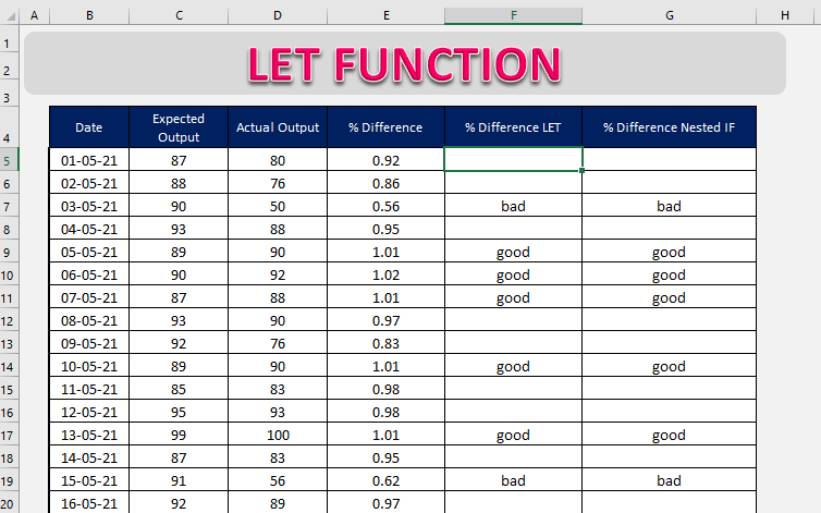
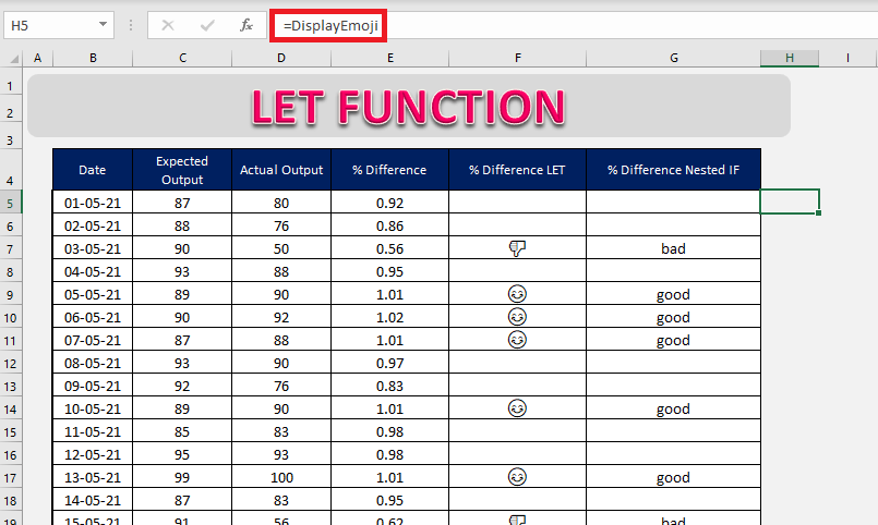
In this example, we have date, expected output, actual output in columns B, C, and D respectively. Since there is a discrepancy between the actual and expected output, we have calculated the difference in percentage between the two in column E.

This will give an estimate regarding how much was actually produced over how much was expected to produce.

• If the difference is less than 0.8, we want to return the word “bad”. It was not a productive day as the units produced was below the expected units.
• If the difference is greater than 1, we want to return the word “good”. It was a productive day as we produced more than what we had expected.

Now, we can use either the Nested IF function or the LET function to achieve this result.

 

Nested IF Function

IF function is used to test a condition and return a value if the condition is met, and a value if it is not. The syntax of the IF function is:

=IF(Logical Test, Value if True, Value if False)

In the example, you will be using the Nested IF function to test both conditions. So, let’s begin!

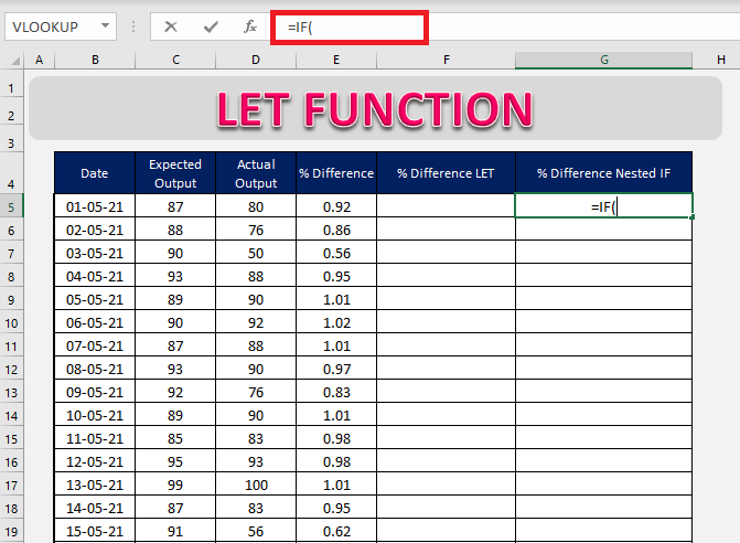
STEP 1: We need to enter the IF function in a blank cell:

=IF(

STEP 2: Enter the first argument – Logical_test

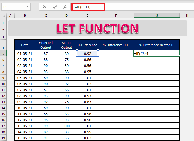
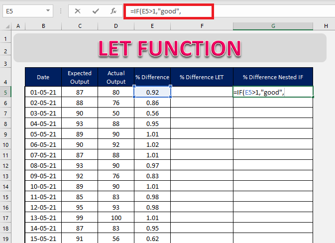
What is your condition? The difference % should be greater than 1.

=IF(E5>1,

STEP 3: Enter the second argument – Value_if_true

What value should be displayed if the condition is true? We want “good” to be displayed.

=IF(E5>1, “good”,

STEP 4: Enter the third argument – Value_if_false

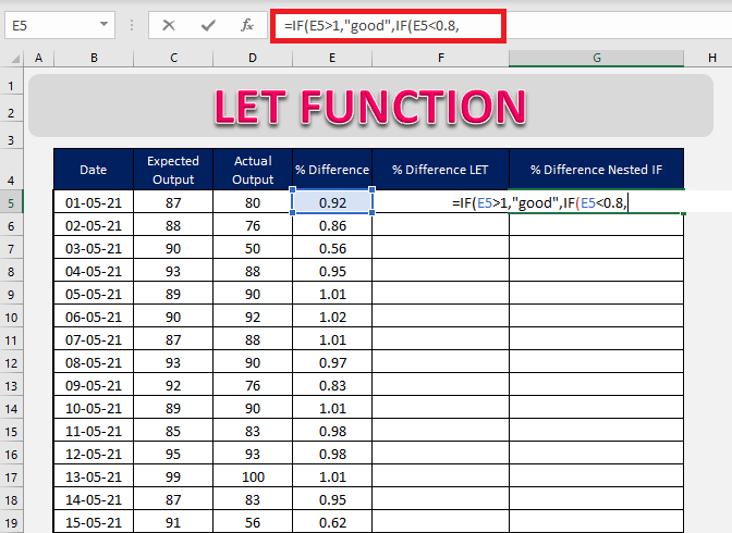
What value should be displayed if the condition is false? If the condition is not met, we want to insert another IF function.

=IF(E5>1, “good”, IF(E5<0.8,

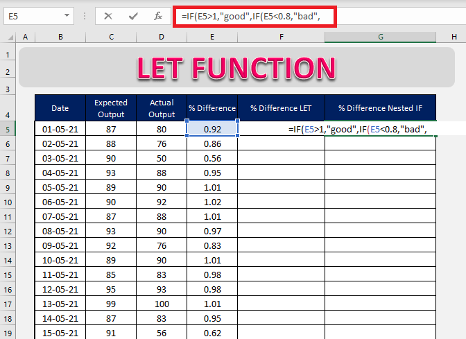
STEP 5: Enter the value if the condition of the second IF function is met.

=IF(E5>1, “good”, IF(E5<0.8, “bad”

 

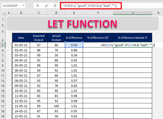
STEP 6: Lastly, enter a blank when both conditions are not met.

=IF(E5>1, “good”, IF(E5<0.8,”bad”,“”)

STEP 7: Copy the formula below in the column.

 

LET Function

In this example, we will assign the difference % to a variable “pchg” using the LET function and then calculate the result.

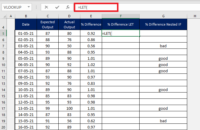
STEP 1: We need to enter the LET function in a blank cell:

=LET(

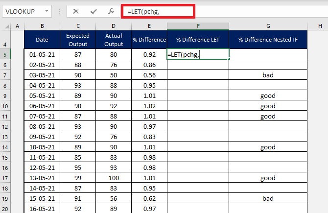
STEP 2: Enter the first argument i.e. name

=LET(pchg,

….

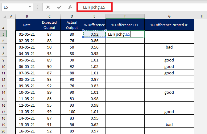
STEP 3: Enter the second argument i.e. value to the name assigned. Here, the value is inserted in cell D5.

=LET(pchg, E5,

STEP 4: Now enter the entire nested IF function and replace the cell reference D5 to the variable pchg.

=LET(pchg, D5, IF(pchg>1,”good”,IF(pchg<0.8,”bad”,””))

As you can see, the LET function does exactly what the IF function was doing when we are using just one variable.

Let’s look at another example where using the LET function will be more useful than the nested IF .function.

 

Example 2:

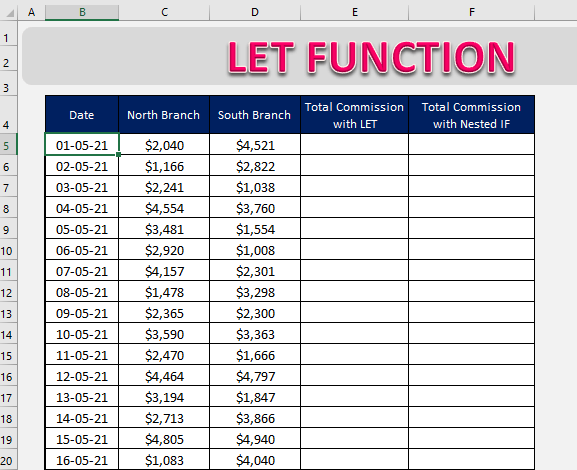
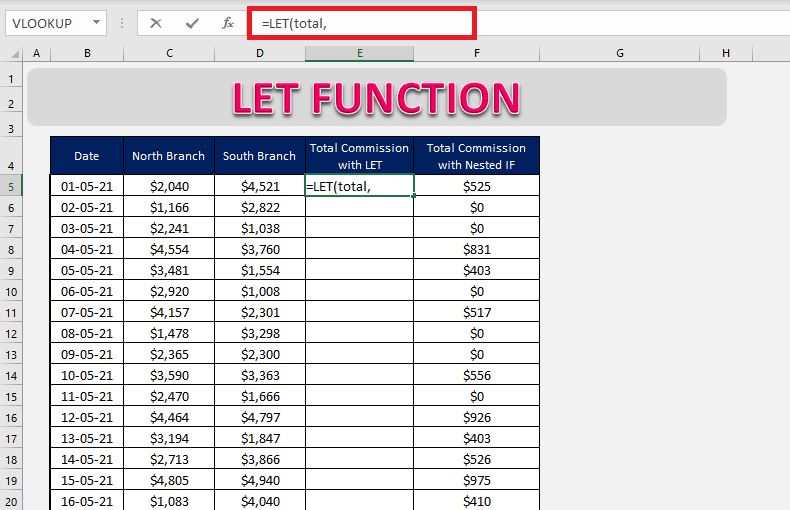
In this example, we have sales from two branches, and we need to calculate commission based on it:

• If the total sales are greater than $7,000, the commission will be 10%;
• If the total sales are greater than $5,000, the commission will be 8%;
• If the total sales are less than or equal to $5,000, the commission will be 0.

In the worksheet below, we have two columns E and F that will contain the commission amount calculated using LET and Nested If respectively.

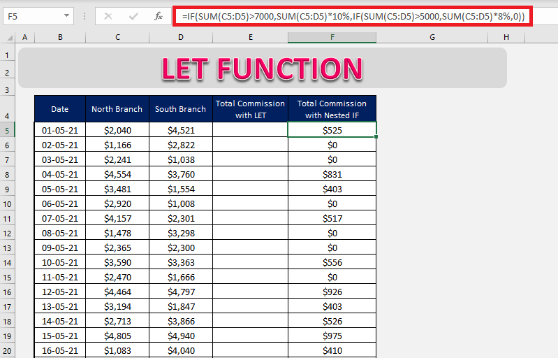
Using the Nested IF function, we can use the following formula to total commission:

=IF(SUM(C5:D5)>7000, SUM(C5:D5)*10%,IF(SUM(C5:D5)>5000, SUM(C5:D5)*8%,0))

Follow the steps below to get the work done using the LET function:

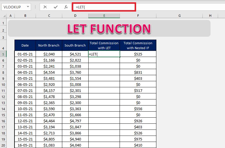
STEP 1: Enter the LET function in a blank cell:

=LET(

STEP 2: Enter the name for the variable to calculate the total sales i.e. total

=LET(total,

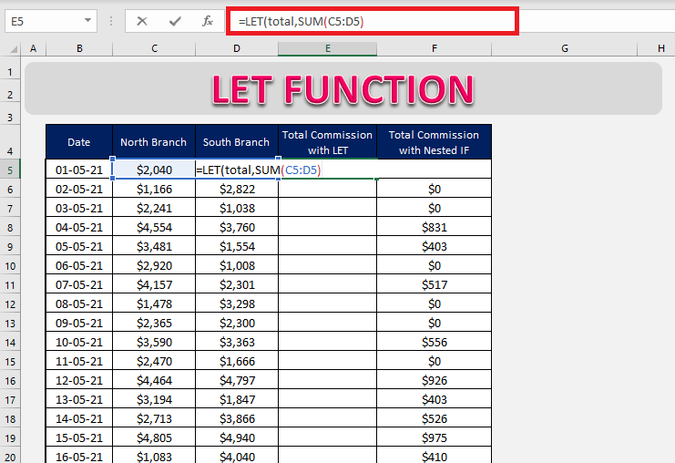
STEP 3: Enter the formula for the defined variable i.e. SUM(C5:D5)

=LET(total, SUM(C5:D5),

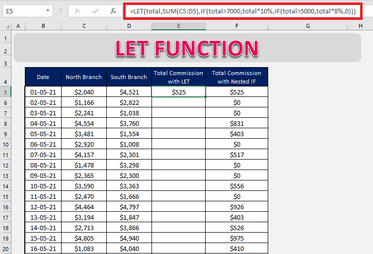
STEP 4: Enter the IF formula using the variable “total”.

=LET(total,SUM(C5:D5), IF(total>7000,total*10%,IF(total>5000,total*8%,0))

If we are using the Nested IF function only, Excel has to calculate the SUM function four times:

=IF(SUM(C5:D5)>7000, SUM(C5:D5)*10%,IF(SUM(C5:D5)>5000, SUM(C5:D5)*8%,0))

Whereas, when we are using the LET function, SUM is calculated just once at the beginning and the calculated value is used in the formula later. This makes the calculation faster and the formula cleaner.

=LET(total,SUM(C5:D5), IF(total>7000,total*10%,IF(total>5000,total*8%,0))

 

Using variables in Excel formulas makes updating the formula quick and easy.  Let’s say we have added another branch in our calculation i.e. West Branch and you need to update the formula.

To do so, simply edit the value of the defined variable from SUM(C5:D5) to SUM(C5:E5) and the total commission will be updated automatically.

=LET(total,SUM(C5:E5), IF(total>7000,total*10%,IF(total>5000,total*8%,0))

 

Until now, we have just used one name-value pair, let’s try using more and see how that works!

 

LET with five name-value pairs

In the previous feedback example instead of using one name-value pair, we will now be using 5.

You can see that there are five variables that we can use in this formula:

• Difference % – pchg
• Percentage you want to check if the difference is good – pergood
• Percentage you want to check if the difference is bad- perbad
• The text you want if the difference is good – textgood
• The text you want if the difference is bad- textbad

 

STEP 1: We need to enter the Excel LET function in a blank cell:

=LET(

STEP 2: Enter the first argument i.e. name of the 1st variable

=LET(pchg,

….

STEP 3: Enter the second argument i.e. value to the name assigned. Here, the value is inserted in cell D5.

=LET(pchg, E5,

 

STEP 4: Enter the name for the 2nd variable i.e. pergood

=LET(pchg, E5, pergood,

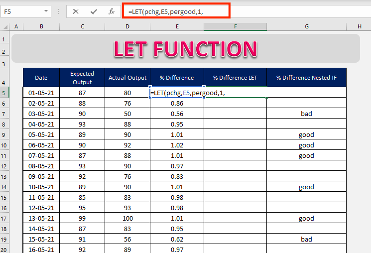
STEP 5: Enter the value for the 2nd variable i.e. 1.

=LET(pchg, E5, pergood, 1,

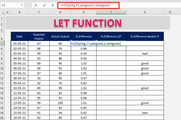
STEP 6: Enter the name for the 3rd variable i.e. textgood

=LET(pchg, E5, pergood, 1, textgood,

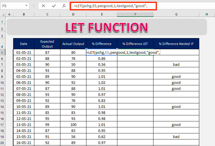
STEP 7: Enter the value for the 3rd variable i.e. “good”. Since it is a text make sure to put it within quotes.

=LET(pchg, E5, pergood, 1, textgood, “good”,

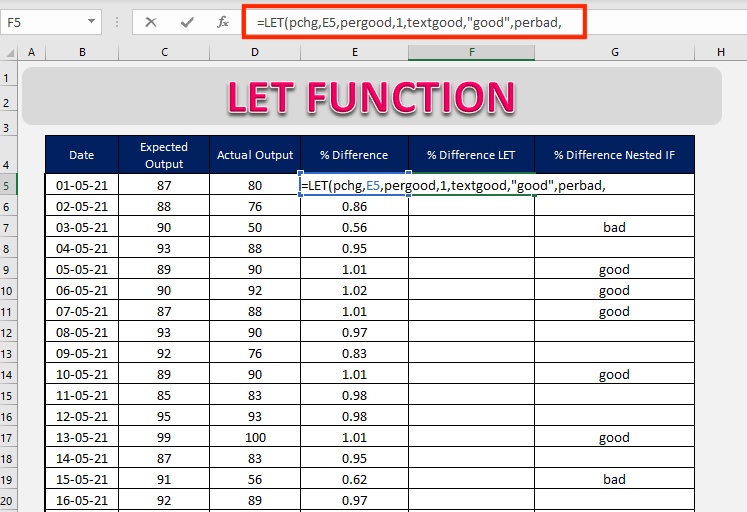
STEP 8: Enter the name for the 4th variable i.e. perbad

=LET(pchg, E5, pergood, 1, textgood, “good”, perbad,

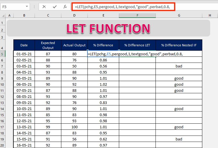
STEP 9: Enter the value for the 4th variable i.e. 0.8

=LET(pchg, E5, pergood, 1, textgood, “good”, perbad, 0.8,

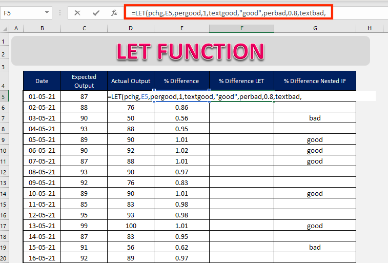
STEP 10: Enter the name for the 5th variable i.e. textbad

=LET(pchg, E5, pergood, 1, textgood, “good”, perbad, 0.8, textbad,

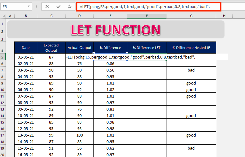
STEP 11: Enter the value for the 5th variable i.e. “bad”

=LET(pchg, E5, pergood, 1, textgood, “good”, perbad, 0.8, textbad, “bad”,

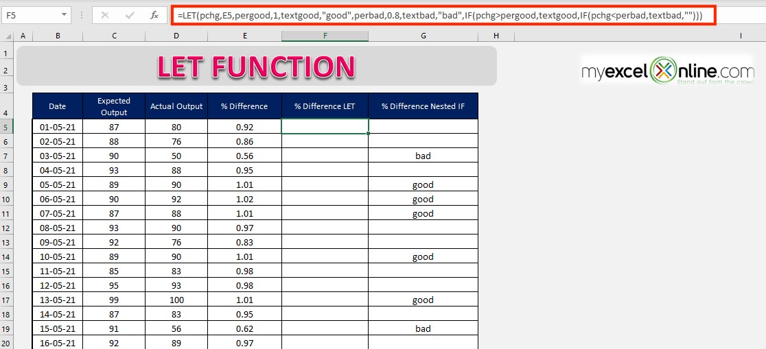
STEP 12: Lastly, enter the nested IF function and replace the cell reference, text, and numbers with the defined variables.

=LET(pchg, E5, pergood, 1, textgood, “good”, perbad, 0.8, textbad, “bad”, IF(pchg>pergood, textgood, IF(pchg<perbad, textbad, “”)))

Copy paste this formula to the remaining cells below.

Using the Excel LET function makes your formula easier to read and update if required in the future.

 

LET with Emojis

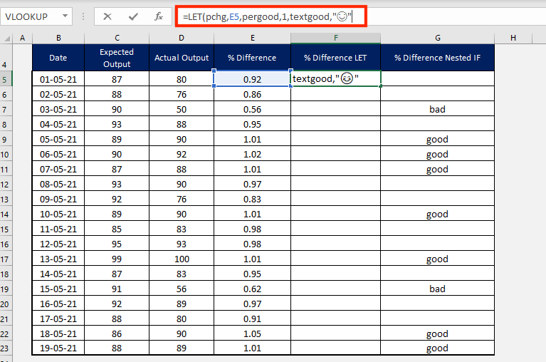
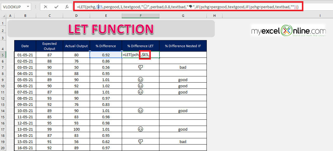
Instead of showing the text “good” or “bad, we can even use emojis. In windows, you can press keys – Windows + . to open the dialog box for emojis and simply click on the one you want to use.

In step 7, replace the text “good” with smile emoji:

=LET(pchg, E5, pergood, 1, textgood,”😊”

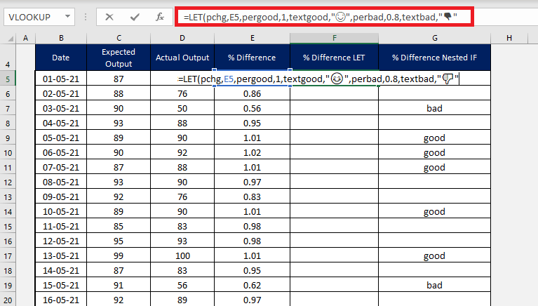
In step 7, replace the text “bad” with a thumb down emoji:

=LET(pchg, E5, pergood, 1, textgood, “😊”, perbad, 0.8, textbad, “👎”

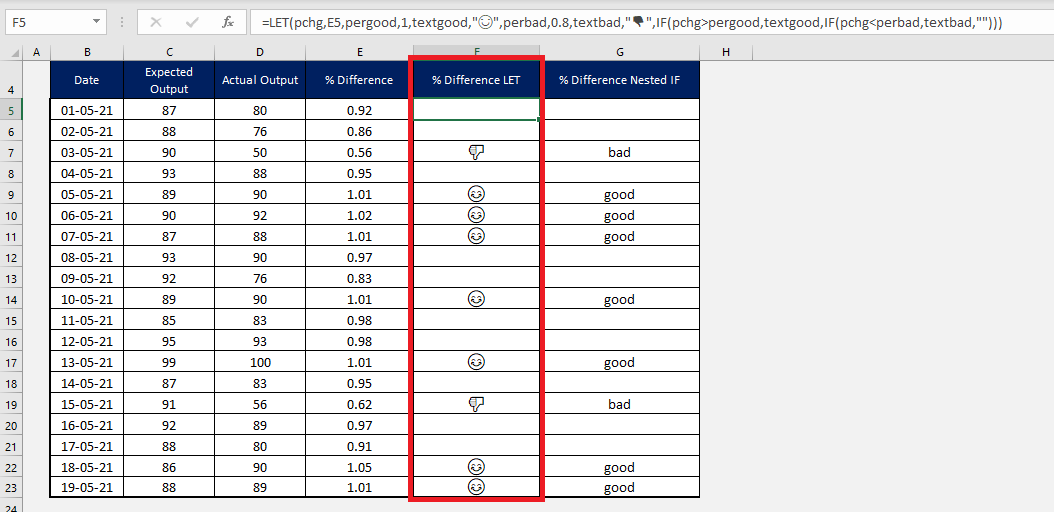
This is what the result will look like. Looks interesting, isn’t it?

=LET(pchg, E5, pergood, 1, textgood, “😊”, perbad, 0.8, textbad, “👎”,IF(pchg>pergood,textgood,IF(pchg<perbad,textbad,””)))

 

LET using Name manager

You can store the long LET formula using name manager and then easily reuse it whenever you want in the future without the need to type the formula again.

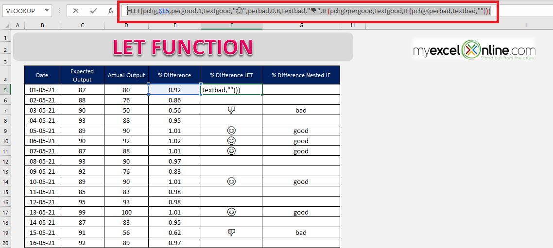
Before we do that, if you look at the formula you will see that column E is a relative reference i.e. if you use this formula the reference will also change. So, if you paste this column in column H, the reference will change from E5 to F5.

But we don’t want that. So, let’s lock column E by putting a dollar sign in front of it.

Now that your formula is ready, follow the steps below to learn how to store it in name manager:

STEP 1: Copy the entire LET formula by pressing the keys Ctrl + C.

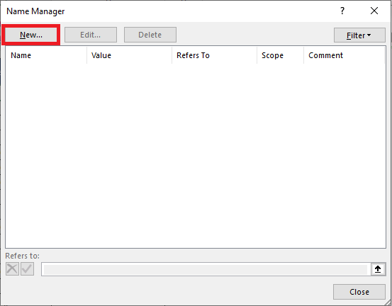
STEP 2: Go to Formula Tab > Name Manager.

STEP 3: In the dialog box, click on New.

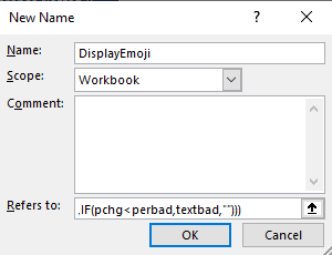
STEP 4: Type the following in the dialog box:

• Name – DisplayEmoji
• Scope – Select Workbook
• Refers to – Paste the formula using Ctrl +V
• Click OK

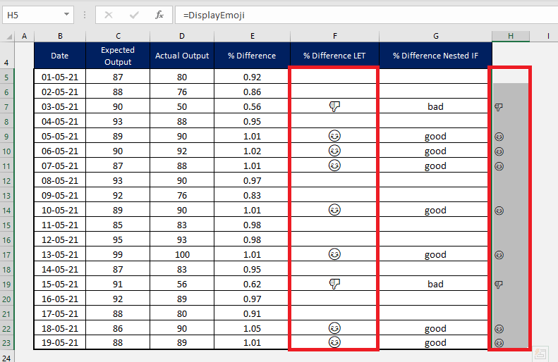
STEP 5: In cell H5, type the function

=DisplayEmoji

STEP 6: Copy-paste the formula below and you will see it is displaying the same result as before.

You can use this formula =DisplayEmoji anywhere in the spreadsheet and it will display the same result!

 

Conclusion

The Excel LET function is a super useful function that helps you eliminate redundancy in a formula and make the formula easy to read and compose. It improves the performance of your spreadsheet since the variables in the Excel formulas are calculated at the beginning and reused later in the formula.

This function is currently available for Office 365 users only. So if you want to use this function make sure to install Office 365 in your system!