The Data Table tool in Excel is a great tool which allows you to run sensitivities on a model in the background. In this article we will show you How to Use the One Variable Data in Excel, as well as the Two-variable Data Table.
Let’s look at these two ways thoroughly!
Download the Excel Workbook below to follow along and understand how to use the One Variable Data and Two Variable Data in Excel –
download excel workbookOneTwo-Variable-Data.xlsx
One Variable Data
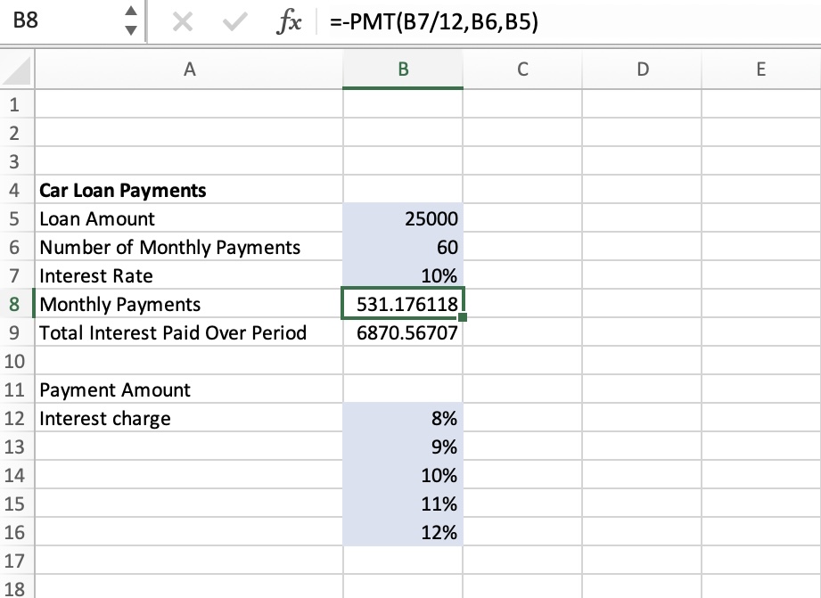
Here we have some data on a very simple spreadsheet to calculate the monthly payment for a loan. We have the >Loan Amount, Interest Rate, Number of Monthly Payments, Monthly Payment, and the Total Interest Paid Over Period.
Use this formula to get the Monthly Payments:
=-PMT(B7/12,B6,B5)
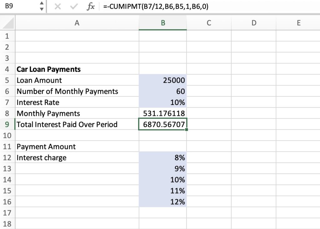
This is the formula to get the Total Interest Paid Over Period:
=-CUMIPMT(B7/12,B6,B5,1,B6,0)
What we want to focus on is the interest rate. Currently, we have it at 10%. We want to find out what our payments will be if it becomes 9%, 8%, 11%, etc.
Manually, we could go and type 8% in the Interest Rate cell to see what the Monthly Payment will be. But if you set up the One Variable Data Table, Excel could do that all for you.
Using this data, we can calculate the Monthly Payments that need to be done.
Let’s set up a column where we will have the interest rates 8%, 9%, 10%, 11%, and 12%. You can do more if necessary.
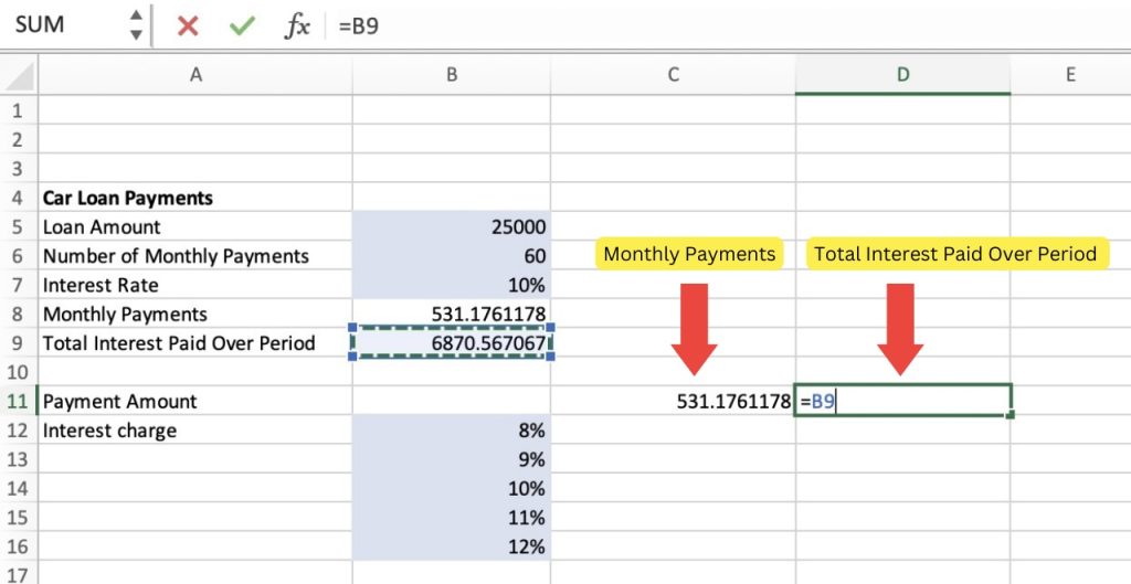
Above our Interest Rate column, and to the right, use = and select the Monthly Payment cell. To the right of that, = it to the Total Interest Paid Over Period.
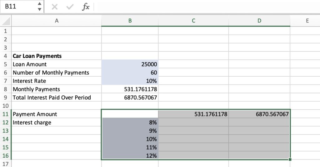
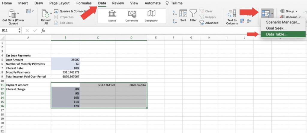
Now, Highlight the outputs at the top (Monthly Payment and Total Interest Paid Over Period), as well as the Interest Rate inputs to the left.
Go to Data, What-If Analysis, Data Table.
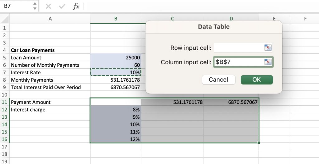
For the Column input cell, Click on the 10% (B7) because together with the formula in cell C11, Excel now knows that it should replace cell B7 with 8% to calculate the Monthly Payment, replace cell B7 with 9% to calculate the Monthly Payment, etc.
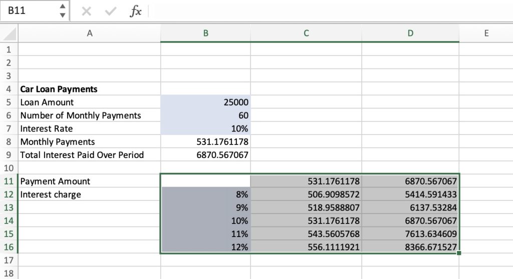
Press OK. It will instantly create a table with the correct figures in correspondence to the Interest Rates.
What’s neat about this Data table is that any change you make on the inputs (the light blue cells) will instantly reflect on the outputs (grey cells).
Conclusion: if the Interest Rate is changed to 8%, the Monthly Payment will be 506.17, if the interest rate becomes 9%, the Monthly Payment becomes 518.95, etc.
Two Variable Data
A Single variable data table is an excellent tool on its’ own. But what if you want to find out what you have to pay in Interest, as well as what the figures are in correlation to the Number of Monthly Payments?
We can achieve this with Data Tables.
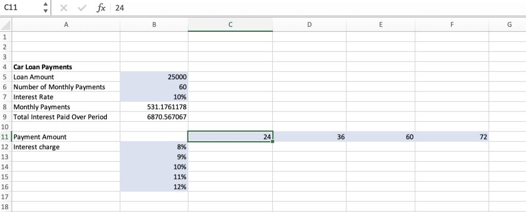
We will set it up by keeping the column of input cells as the Interest charge.
Above, and to the right, input your Number of Monthly Payments.
Now, the output cell has to above the Interest Rate inputs. Press = then click on the Monthly Payment cell (B8).
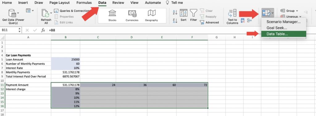
Highlight the table, making sure to include the input and the output.
Go to Data, What-if Analysis, then Data Table.
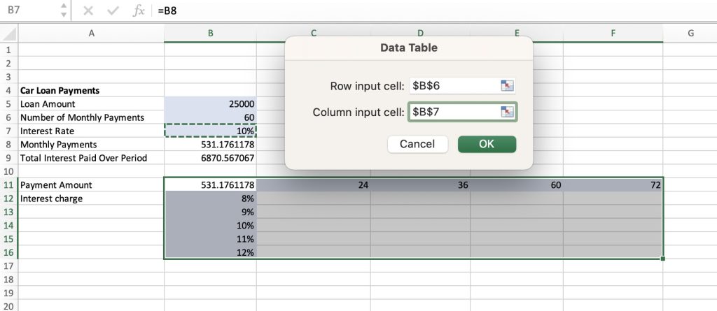
For the Row input cell, press the Number of Monthly Payments cell. For the Column input cell, press the Interest Rate cell.
Click OK.
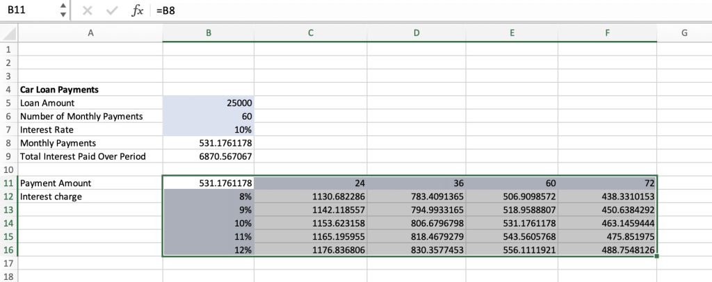
As you can see, it will show you what the Monthly Payments will be at 24 months at 8%, 36 months at 11%, etc.
There you have it! By setting up your data correctly, defining the input cell, and creating the One Variable Data Table, you can quickly and easily analyze the impact of different input values on the result. Whether you’re analyzing financial data or any other type of data that involves input variables, One Variable Data Tables can help you make better decisions based on your data.
John Michaloudis is a former accountant and finance analyst at General Electric, a Microsoft MVP since 2020, an Amazon #1 bestselling author of 4 Microsoft Excel books and teacher of Microsoft Excel & Office over at his flagship MyExcelOnline Academy Online Course.

