2 Quick Methods to Use IF Statements & Drop Down Menu in Excel

Microsoft Excel‘s IF statement is a versatile tool that allows users to perform conditional logic, effectively enabling decisions within spreadsheets based on criteria. Combining this with a drop down menu can elevate data entry to a more dynamic and responsive level, where choices in one menu influence the options available in another, streamlining the user’s interaction with data sets like varying wedding lists.

Key Takeaways

• Dropdown is a feature that allows you to create a list of predefined options from which users can choose when entering data into a cell
• The IF statement is integral to creating conditional drop-down lists in Excel, allowing the display of different lists based on user selection.
• Direct cell references or named ranges can be utilized alongside IF statements to craft dynamic drop-down menus with varying content.
• Advanced Excel users can streamline the conditional list creation using the IF/IFS function for situations with single or multiple conditions.

 

Download the Excel workbook and follow along with the tutorial on How to Create IF Statements & Drop-Down Menu in Excel – download excel workbookDrop-Down-Menu.xlsx

 

Introduction to Streamlining Data with IF Statements and Drop-Downs in Excel

The Power of IF Statements in Data Organization

Microsoft Excel provides an extensive range of functions to manage and organize data effectively. At the forefront of these is the IF statement—a powerful tool that evaluates conditions and makes logical comparisons to return specific values. Its use ranges from simple checks to complex decision-making scenarios within your datasets.

The Role of Drop-Down Lists in Efficient Data Entry

Drop down lists are a staple in the Excel toolbox for ensuring data consistency and saving time on data entry. Users can choose from a pre-established set of options. rather than entering data manually, which minimizes the risk of errors and standardizes entries across your spreadsheet.

Especially useful in forms, surveys, and dashboards, drop-down lists streamline workflows and enhance the user experience by providing clear, selectable choices.

 

Enhancing Usability with Excel Drop-Down Lists

Steps to Create Basic Drop-Down Lists using Data Validation

Creating basic drop-down lists in Excel is a straightforward process that can be achieved using the Data Validation tool. Here’s how to set up a simple drop-down list:

STEP 1: Source Data Preparation.

Create a compilation of the options you wish to incorporate into your dropdown. Input them either in a column or row within your worksheet or in a separate one.

STEP 2: Select the Data Entry Cell.

Select the cell in which you’d like the drop-down list to be displayed; usually, this will be the cell where users enter data using the drop-down menu.

STEP 3: Access Data Validation Settings.

Navigate to the Data tab and within the Data Tools group, select ‘Data Validation.

STEP 4: Set Up the Drop Down Menu

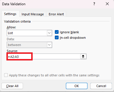
• In the Data Validation dialog box, under the ‘Settings’ tab, find the ‘Allow’ field and select ‘List’ from the drop-down menu.
• In the ‘Source’ box that becomes active upon selecting ‘List’, enter the range of cells containing your options (e.g., A2:A3), or enter the values directly separated by commas.
• Ensure the ‘In-cell dropdown’ option is checked to display the arrow for the drop-down list.

STEP 5: Customize with Optional Messages.

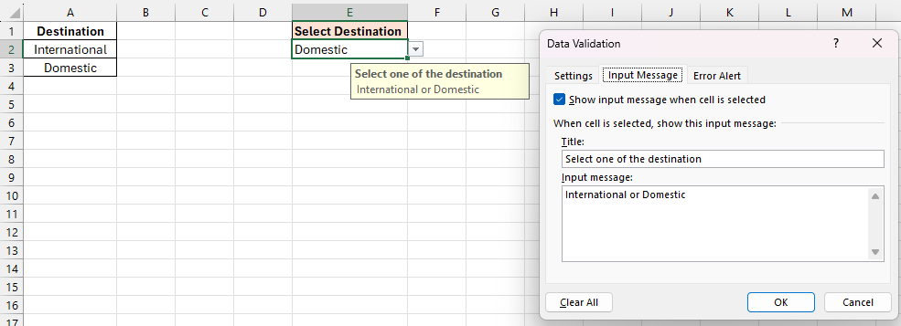
• In the ‘Input Message’ tab, you have the option to generate a message that will display when the cell is chosen, providing guidance to users on their selection.

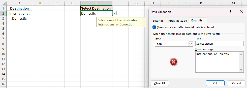
• Under the ‘Error Alert’ tab, you can configure warning messages to show when an incorrect entry is made.

STEP 6: Complete and Test.

Click ‘OK’ to confirm the data validation settings. Test the drop-down by clicking on the cell with the drop-down list and selecting an option from the list that appears.

This simple drop-down list will now help users choose from the predefined set of options, ensuring data consistency and accuracy.

 

Advancing to Dynamic Drop Down Menu

Creating dynamic drop-down lists in Excel can be an extremely helpful feature when dealing with interdependent data. Here are three effective methods to create dynamic drop-down lists using the IF function and the IFS function.

Method 1 – Using the IF Function

Using IF statements in conjunction with drop-down lists can create a conditional selection environment that adapts based on user input elsewhere in the spreadsheet. Here is a guide to refining drop-down list options with IF statements:

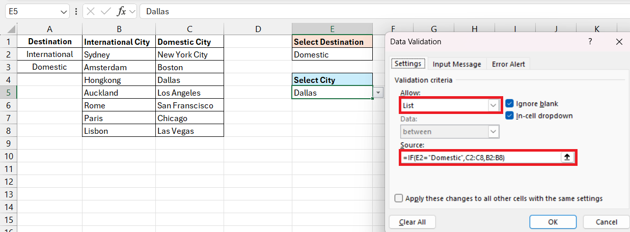
STEP 1: Determine what the condition is and which cell will trigger the change (for instance, a cell where the user selects “Domestic” or “International”).

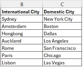
STEP 2: Prepare two lists that correspond to the condition. For example, one list for domestic options and another for international options.

STEP 3: Select the cell where you’d like the conditional drop-down list to appear and go to ‘Data’ > ‘Data Validation’.

STEP 4: In the Data Validation dialogue box, select ‘List’ in the ‘Allow’ field and in the ‘Source’ box, enter your IF statement referencing the condition cell and the named lists. For instance: =IF(E2=”Domestic”,C2:C8,B2:B8).

By incorporating IF statements with your drop-down lists, you have harnessed Excel’s capability to create a dynamic and user-interactive workbook that can respond intelligently to the context of data entered.

 

Method 2 – Using the IFS Function

In this example, you have to create a list of dependent options as before but for multiple categories. Each category will align with a different condition within the IFS function. Use the IFS function to evaluate multiple conditions at once. This results in a cleaner formula compared to multiple nested IF statements.

For instance, the Data Validation formula might be `=IFS(E2=”Beaches”,$B$2:$B$8,E2=”Mountains”,$C$2:$C$8,E2=”Urban Areas”,$D$2:$D$8)` for an input cell E2 and corresponding locations for every destination category.

 

Create Drop Down Menu Using Named Ranges

Named ranges in Excel not only declutter your formulas but also enhance clarity and reduce errors. They allow you to assign meaningful names to individual cells, ranges of cells, formulas, or constants. Here’s how to use named ranges to simplify your Excel formulas:

STEP 1: Choose the cell or range of cells you want to assign a name to.

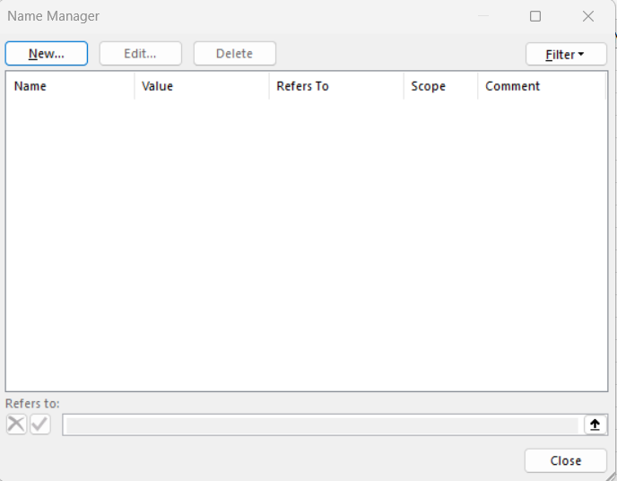
STEP 2: Go to the Formulas tab, click on ‘Name Manager’, and then ‘New’.

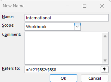
STEP 3: Enter a meaningful name in the ‘Name’ field and specify the scope. Excel names cannot include spaces and must start with a letter or underscore.

STEP 4: Instead of using cell references like B2:B8 and C2:C8, use the named range International and Domestic respectively directly in formulas. This simplifies understanding the formula’s purpose and makes editing easier.

Use named ranges to organize and categorize data, which is especially useful when dealing with complex models or large datasets. Named ranges make it quicker to navigate large workbooks.

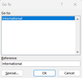
By using the ‘Name Box’ or ‘Go To’ command (Ctrl + G), you can instantly jump to the specified range.

Named ranges improve the readability of formulas by replacing obscure cell references with descriptive names, making the workbook more maintainable and shareable.

Named ranges are a component of best practices for Excel usage and are particularly useful for frequently referenced data and for ensuring that your Excel formulas remain intelligible and manageable.

Remember that consistency in naming conventions and keeping track of named ranges are crucial to maintaining an organized and efficient Excel environment.

 

Real-World Examples of Conditional Drop-Down Menu

Conditional drop-down menu can significantly improve data entry accuracy and user experience in various real-world applications. Here are some examples where such lists can be particularly useful:

• In an order form, users might need to select a product category before choosing a specific product. Conditional drop-down lists ensure that only relevant products are displayed based on the selected category.
• When onboarding new employees, HR forms might require selecting a department first, which could then restrict the job title options to those pertinent to the selected department.
• In inventory sheets, selecting a main inventory category, such as ‘Electronics’, could lead to a secondary drop-down showing only items like ‘Laptops’, ‘Monitors’, and ‘Keyboards’, making stock management more controlled and efficient.
• For financial reports, choosing a particular quarter might conditionally allow for further selection of monthly data within that quarter, ensuring data consistency in time-sensitive reporting.
• In educational portals, selecting a particular course could dynamically update a secondary drop-down with the available classes or sections, streamlining the enrollment process for students.
• Surveys often use conditional drop-down lists to ask follow-up questions specific to a respondent’s prior answers, maintaining relevance and clarity throughout the survey.
• Project management tools may have drop-down lists that first require the selection of a project before displaying a list of associated tasks or milestones specific to it.

These examples showcase how conditional drop-down lists can help manage data effectively across different fields, making Excel a powerful tool for organizers, administrators, and analysts who desire to maintain structured and reliable datasets.

 

Overcoming Challenges and Tips for Best Practices

Troubleshooting Common Issues with IF Statements and Drop-Downs

Even with careful planning and design, Excel users may encounter issues when working with IF statements and drop-down lists. Here are some common problems and how to troubleshoot them:

Issue: The IF statement returns unexpected results or errors.

Solution: Double-check the logic of your IF statement. Ensure that all conditions are correctly stated and that you’ve used the proper syntax. Use the F9 key to evaluate parts of your formula.

Issue: The expected drop-down arrow is not showing in the cell.

Solution: Ensure that the ‘In-cell dropdown’ option is enabled in the Data Validation settings, and check that the cell is not protected or part of a locked sheet.

Issue: The drop-down list is visible, but no data appears when clicked.

Solution: Verify the source range for the list in Data Validation. If you’re using a dynamic source or the INDIRECT function, ensure that the named ranges or formulas are correctly defined.

Issue: Users can enter values that are not part of the drop-down options.

Solution: Within the Data Validation dialog box, access the ‘Error Alert’ tab and enable the ‘Show error alert after invalid data is entered’ option to discourage inaccurate entries.

Issue: The drop-down list is hard to see or use due to formatting.

Solution: Adjust the cell formatting, theme, or styles that may be impacting the visibility of the drop-down list, ensuring sufficient contrast and clear fonts.

When dealing with these issues, patience and a methodical approach to checking your formulas and data validation settings can go a long way.

 

FAQ – Excel IF Statements and Drop-Down Lists

What are the benefits of using an IF statement in a drop-down list?

Utilizing an IF statement in a drop-down list offers several advantages that can enhance the functionality and user experience of an Excel spreadsheet:

1. Dynamic Content: IF statements can alter the contents of a drop-down list based on user input or other conditions, making the list responsive and interactive.
2. Improved User Experience: Conditional drop-down lists simplify the user interface by reducing clutter, showing only the options that are pertinent to a user’s prior selections.
3. Streamlined Data Entry: Users are guided through a logical sequence of choices, streamlining the data entry process and reducing time required for input.
4. Data Management: IF statements can help in managing large sets of data by breaking them down into more manageable, context-specific options.

How can I use dynamic ranges to make my drop-down list more adaptive?

Dynamic ranges can be used for creating flexible drop-down lists that automatically adjust as the data changes. You can use IF function, IFS functions and Names ranges to create dynamic ranges.

How do I create criteria for a drop-down list in Excel?

To create criteria for a drop-down list in Excel, select the cell where you want the drop-down menu, go to the “Data” tab, choose “Data Validation,” and set the criteria under the “Settings” tab. Specify the criteria in the “Allow” dropdown menu, such as “List” or “Whole Number,” and provide the corresponding values or range to establish the criteria for the drop-down list.

Can you use an IF function for a drop-down list?

Yes, you can use an IF function to determine the contents of a drop-down list in Excel. The IF function can serve to create a conditional drop-down list where the options presented to the user change based on another input or condition within the workbook.