Excel IFNA Function: Your Ultimate Tool for Error Handling

Microsoft Excel‘s IFNA function acts as a strategic safety net within its suite of error-handling tools, ensuring that your data analysis remains unscathed when confronted with the common #N/A error. It provides a seamless way to substitute a more meaningful or neutral value in place of errors, maintaining the integrity and clarity of your datasets.

Key Takeaways:

• Targeted Error Handling: IFNA specifically addresses #N/A errors, allowing for precise error management in formulas.
• Syntax Simplicity: Use IFNA by specifying the value to check and the replacement for an #N/A error using IFNA(value, value_if_na).
• Integration with VLOOKUP: Pair IFNA with VLOOKUP to handle missing data gracefully, replacing potential #N/A errors with a predefined alternative.
• Comparison with IFERROR: Choose IFNA for #N/A errors for specificity or IFERROR for a broader error catchment, depending on your needs.
• Alternatives for Broader Errors: Explore other functions like ISERROR or ISERR when expecting a range of error types, allowing for more tailored error handling strategies.

 

Introduction to IFNA in Excel

Navigating Through Excel’s Error Handling Functions

Diving into Excel’s vast functionality, you’ll discover a suite of error-handling tools designed to make your data analysis as smooth as sailing. They’ve put a safety net under your data circus, ensuring that if your formulas walk the tightrope and fall, there’s a way to catch them gracefully.

What is IFNA function?

The IFNA function is like having a plan B in place, standing ready for those moments when Excel stumbles upon the notorious #N/A error—a signal that a value is not available. It’s a clever way to ensure that, instead of an error message that could throw your data analysis off-track, you get a predefined substitute that keeps everything on the right path. Introduce IFNA into your spreadsheet, and you’ll find it a reliable ally in maintaining data integrity and clarity.

The Anatomy of the IFNA Function

Understanding the IFNA Syntax

Getting to grips with the IFNA function syntax is like learning a simple magic spell for your data woes. The formula follows a straightforward structure: IFNA(value, value_if_na).

You cast this spell by specifying two things – the value you’re scrutinizing for the sneaky #N/A error and the value you wish to summon in its place if that error arises. It’s as if you’re saying to Excel, “If this turns out to be an error, here’s what I’d like you to do instead.”

Parameters Explained for Clarity

The IFNA function smoothly operates with just two simple components under its hood:

• value: This is the formula you need evaluated – the trick you’re undertaking that might end in an #N/A error. Think of it as the conjuring part of a magic act, where something might just disappear.

• value_if_na: This is your safety net – the alternative result you want Excel to pull from its hat if the value turns out to be #N/A. It’s the comforting presence that ensures your performance never falters.

Think of these parameters as partners in a dance, where one takes a bold step and the other gracefully follows if the first one stumbles.

Practical IFNA Applications

Combining IFNA with VLOOKUP for Seamless Lookups

Integrating IFNA with VLOOKUP is like equipping your lookup missions with a safety harness. When your usual VLOOKUP formula is sent out to match data across tables, wrap it in the embrace of an IFNA. This two-step combo ensures that if VLOOKUP draws a blank and #N/A appears, IFNA will cover for it, presenting a cleaner, alternative result of your choice instead of an error.

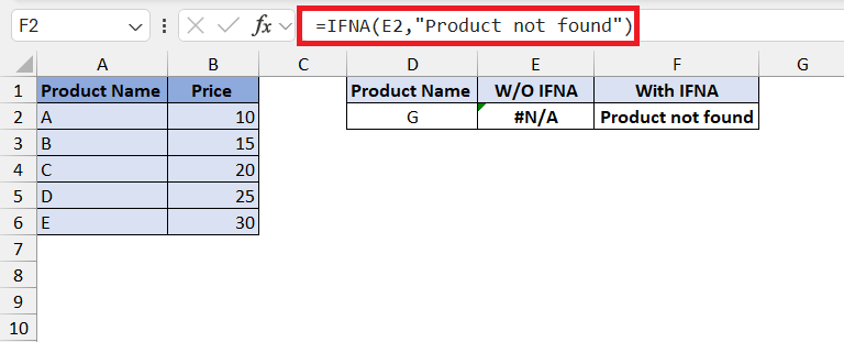
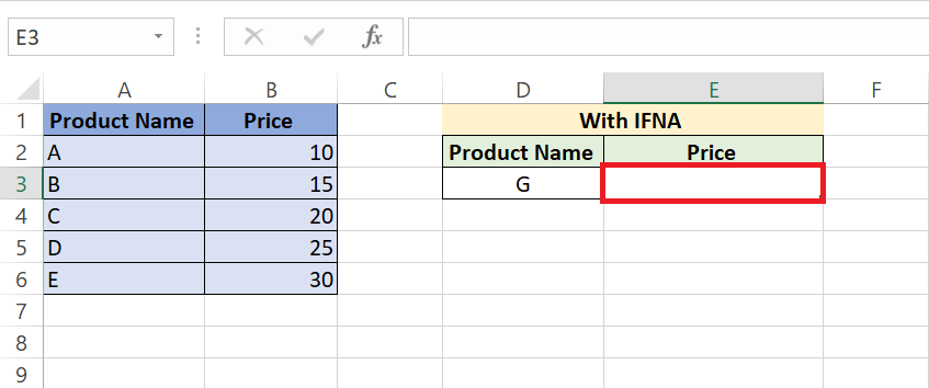
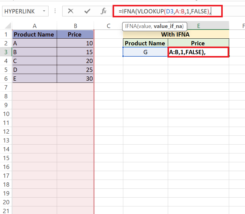
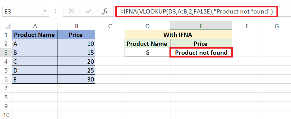
Let’s say you have a dataset in Excel with two columns: A for Product Names and B for their corresponding Prices. You want to look up the price of a product, but if the product is not found in the list, you want Excel to return “Product not found” instead of showing the #N/A error. Here’s how to use it with a dataset of product names and prices:

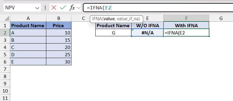
STEP 1: Select a Cell: Choose where you want the result.

STEP 2: Enter Formula: Type “=IFNA(” and insert a formula, like VLOOKUP or INDEX/MATCH, referencing your dataset: “=VLOOKUP(A2, A:B, 2, FALSE)”.

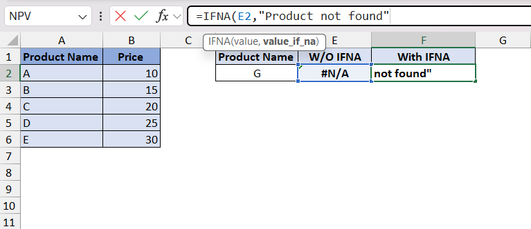
STEP 3: Close Formula: Add “, ” then specify a value to display if the formula returns #N/A, like “Product not found”. Close the formula with “)” and press Enter.

Not only does this partnership maintain the aesthetic of your data, but it also can navigate sequential or chained lookups across different sheets, working like a relay race where IFNA hands off the search to the next VLOOKUP, until there are no more lookups or, voila, a match is found!

Comparing IFNA with Its Cousins

IFNA vs. IFERROR: Choosing the Right Tool

Imagine you’re choosing tools from a toolbox – IFNA and IFERROR each have their specific uses. Choose IFNA when you want to deal exclusively with the #N/A error, giving you the precision akin to using a scalpel—ideal for fine-tuning your data when you’re certain that #N/A is the only hiccup possible.

On the other hand, IFERROR is the Swiss Army knife, catching all types of errors without discrimination. This could be perfect when you want to cast a wider safety net, especially when various errors could pop up, and you’d rather have a general fix ready.

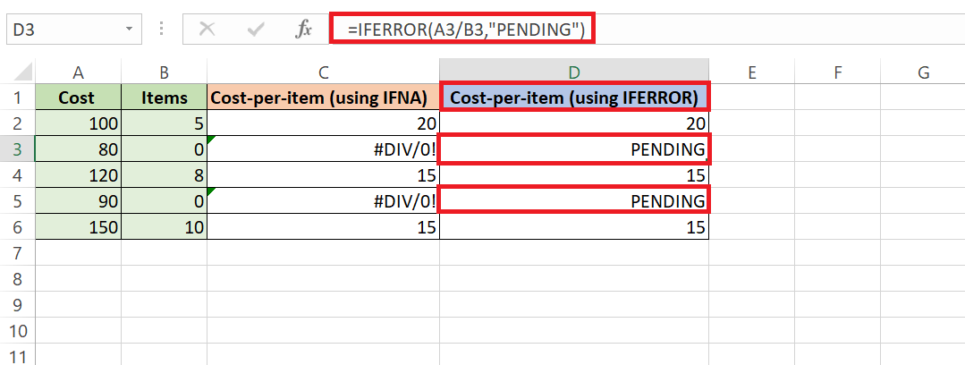
Let’s take an example when calculating the cost-per-item and anticipating potential division errors due to items not being shipped, IFERROR can be employed to gracefully manage these situations. Unlike IFNA, which specifically targets the #N/A error, IFERROR handles any type of error, including division errors. By incorporating IFERROR into the formula, such as “=IFERROR(Cost/Items, “Pending”)”, Excel will display “Pending” whenever a division error occurs, effectively mitigating the risk of encountering disruptive errors in the cost-per-item calculation.

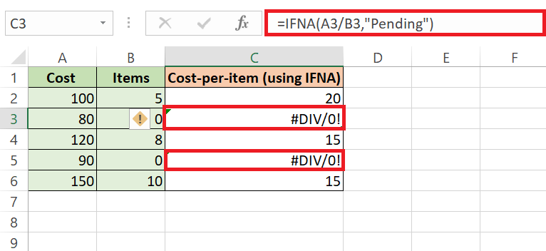
CASE 1: The IFNA function can only handle NA errors and not any other types of errors like #DIV/0!.

CASE 2: The below shows how the division error can be mitigated by using IFERROR function.

Deciding between the two hinges on the particular errors you’re expecting to encounter. If you’re looking for a focused solution, IFNA is your go-to, whereas, for a more all-encompassing approach, IFERROR stands out.

Alternatives to IFNA for Different Situations

If IFNA doesn’t quite fit your scenario, fret not – Excel offers a smorgasbord of alternatives for different error-handling appetites. For pre-2013 Excel enthusiasts, knitting together IF with ISNA mimics IFNA’s functionality, catching those #N/A errors with a homemade feel. When your data forecast predicts a broader range of errors, IFERROR might be the umbrella you need.

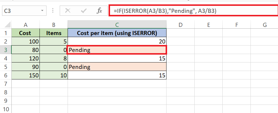
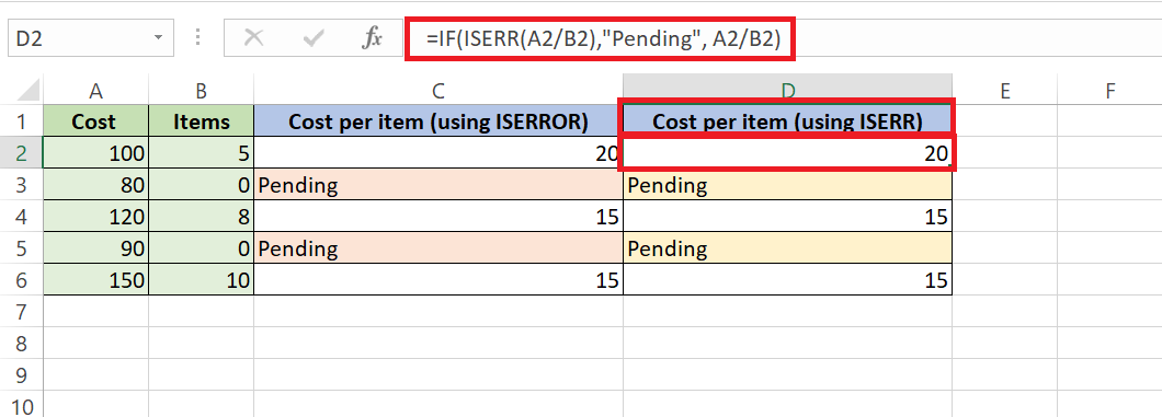
In the context of the cost-per-item calculation where division errors might occur due to items not being shipped, utilizing the ISERROR or ISERR functions provides more precise control over error handling. Unlike IFERROR, which handles any type of error generically, ISERROR and ISERR allow for specific identification and treatment of division errors. Here’s how they could be integrated into the formula:

=IF(ISERROR(Cost/Items), “Pending”, Cost/Items)

Alternatively,

=IF(ISERR(Cost/Items), “Pending”, Cost/Items)

This formula checks if the division operation results in an error. If it does, “Pending” is displayed; otherwise, the cost-per-item is calculated and shown. ISERR can also be used similarly, but it’s slightly less inclusive than ISERROR, excluding some less critical errors.

For more granular control, tapping into ISERROR or ISERR could be akin to choosing the manual gears over an automatic transmission, giving you the chance to address specific error types individually.

And for the lovers of pristine data who prefer warnings over substitutions, conditional formatting offers a visual flare that highlights rather than hides errors.

Every tool has its moment to shine – it’s all about having the wisdom to choose the appropriate one for the task at hand.

Frequently Asked Questions (FAQs)

Q: What is the difference between ISNA and IFNA?

A: ISNA detects the #N/A error in Excel and returns “TRUE” if found, otherwise it’s “FALSE”. IFNA catches the same error but lets you replace it with a value you choose, for clearer data presentation. ISNA is the lookout, while IFNA is both the lookout and the problem solver.

Q: How to use IFNA with VLOOKUP?

A: To use IFNA with VLOOKUP, nest your VLOOKUP formula inside an IFNA function like this: =IFNA(VLOOKUP(lookup_value, table_array, col_index_num, [range_lookup]), "Custom Error Message"). This way, if VLOOKUP returns #N/A, IFNA will show your custom message instead.

How do I use the IFNA function in Excel?

A: Use the IFNA function in Excel by writing =IFNA(value, value_if_na) in a cell, where value is the expression you’re examining, and value_if_na is what you want to show if Excel finds an #N/A error in value.

How do I use Vlookup and IFNA together?

A: Combine VLOOKUP and IFNA by enclosing the VLOOKUP function inside IFNA: =IFNA(VLOOKUP(lookup_value, table_array, col_index_num, [range_lookup]), "Alternate Value"). This provides an error-free result if VLOOKUP encounters an #N/A error.

What if IFNA is an empty cell in Excel?

A: If the value or value_if_na in an IFNA function is an empty cell, Excel treats it as an empty string (“”). So, =IFNA(A1, B1) would return an empty string if A1 or B1 are empty and A1 has an #N/A error.