Index in Excel Pivot Tables

One cool thing with Excel is you are able to show values as the Index in Pivot Table. In a nutshell, the Index will tell you the relative importance of a cell i.e. it will show you the relative importance of each value when compared to its row, column, and grand total. It can help you make decisions if, for example, you want to increase the price of your product, then you will be able to identify the area that will be most impacted (based on the Index).

Key Takeaways:

• Purpose of the Index Value: The Index function in Pivot Tables measures the relative importance of a value within the table. It shows how much more (or less) significant a specific data point is compared to the overall data distribution.
• Formula Behind Index: The Index value is calculated using the formula:
  (Value in Cell × Grand Total) ÷ (Row Total × Column Total). This calculation ensures that the Index adjusts for the size of the row and column totals, providing a normalized measure of significance.
• Use Case for Index: The Index is particularly useful in large data sets where simple percentages or raw totals don’t highlight significant patterns. It’s great for analyzing outliers or identifying areas where performance is above or below expectations.
• Setting Up Index in Pivot Tables: To use the Index calculation, right-click a value in the Pivot Table, select Show Values As, and choose Index. Excel will then display the normalized values based on the Index formula.
• Interpreting Index Values: An Index value of 1 indicates that a data point is proportional to its row and column totals. Values greater than 1 signify higher-than-expected importance, while values less than 1 indicate lower-than-expected importance in the overall dataset.

Index in Excel Pivot Tables

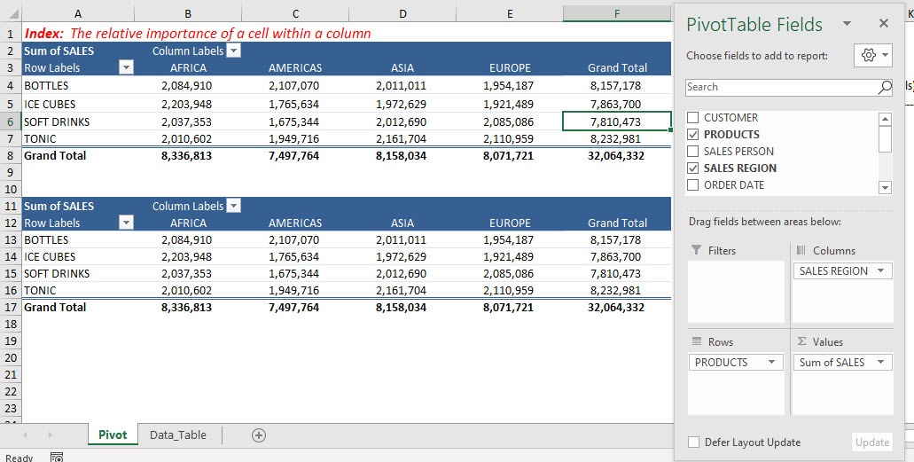
STEP 1: Here is our Pivot Table. The two tables are exactly the same.

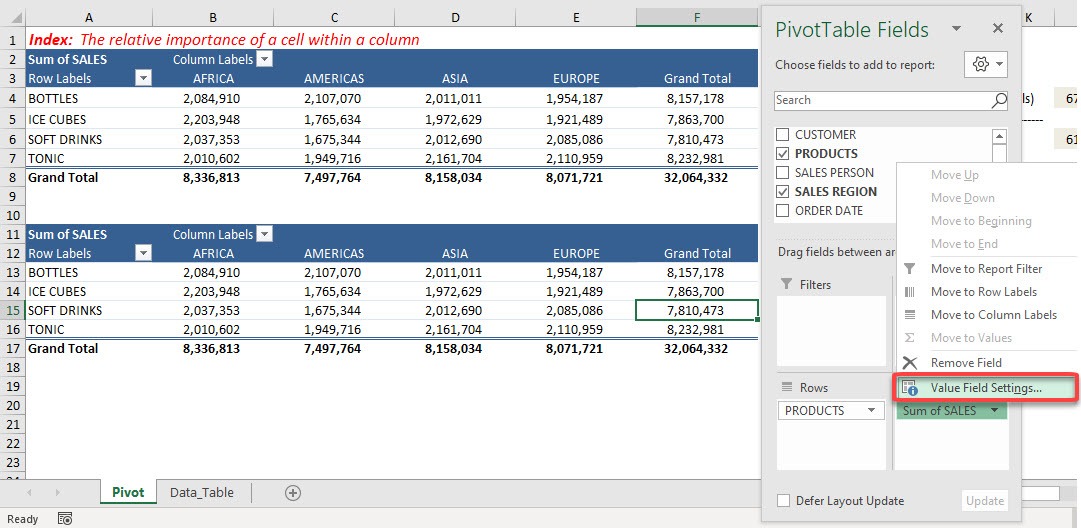
STEP 2: Go to the second Pivot Table, and click on the arrow of Sum of SALES and select Value Field Settings

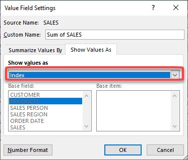
STEP 3: Select Show values as > Index. Click OK

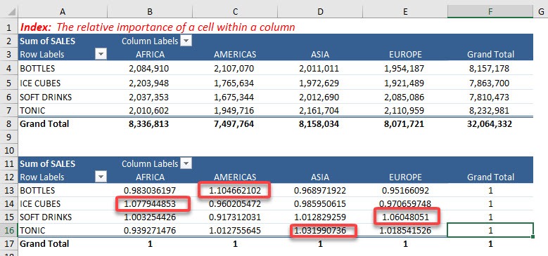
STEP 4: Now we have our Index values! The higher value means that it is the most important value for that column, for example, Bottles have the greatest impact on the Americas Region in terms of sales.

Now let’s have a quick calculation to show how Index is calculated. Let us target the Bottles Sales for the Americas Region.

STEP 5: Select the Sales for Bottles-Americas then multiply it by the Grand Total.

STEP 6: Multiply the Grand Row Total of Bottles and the Grand Column Total of Americas.

STEP 7: Divide them and you will get the Index!

The values are exactly the same!

Quick Explanation of the Numbers

Thus, you can calculate the index number for any value by using the formula below:

= (Value of cell * Grand total of Grand Totals) / (Grand Row Total * Grand Column Total)

In this example, you can see that the sales amount of bottles in Africa (2,084,910) and soft drinks in Europe (2,085,086) are almost equal.

But, the index numbers are 0.98 and 1.06.

The reason behind this difference is that grand total of Africa is greater than that of Europe. So, when the Africa bottles sales amount is divided by a larger number, it results in a lower index number.

These index numbers give the user a clear picture of the importance of each sales amount as per the row, column, and grand totals. The following should be noted with respect to the index number:

• If all the values in the Pivot Table are equal, the index in Pivot Table will be 1.
• If the index in Pivot Table is less than 1, it means that the value is of lower importance than its row and column values.
• If the index in Pivot Table is greater than 1, it means that the value is of greater importance than its row and column values.

Frequently Asked Questions

What is the purpose of the Index function in Pivot Tables?
The Index function measures the relative importance or significance of a specific value in the Pivot Table compared to the overall data distribution. It normalizes data points to help identify patterns, outliers, or areas of interest.

How is the Index value calculated in Pivot Tables?
The Index value is calculated using the formula: (Value in Cell × Grand Total) ÷ (Row Total × Column Total). This ensures that the Index accounts for the proportions of the row and column totals, providing a fair comparison.

When should I use the Index calculation in a Pivot Table?
The Index calculation is ideal when you want to highlight areas of significance within large data sets or compare values proportionally rather than just using raw totals or percentages. It’s especially useful for advanced analysis, like identifying outliers or trends.

How can I apply the Index function in a Pivot Table?
To apply the Index function, right-click on any value in the Pivot Table, select Show Values As, and choose Index. Excel will then display the normalized Index values in the table.

How should I interpret the Index values?
An Index value of 1 indicates a proportional or expected significance for that data point. Values greater than 1 mean the data point is more significant than expected, while values less than 1 indicate lower significance relative to the row, column, and overall totals.