Index Match 2 Criteria with Data Validation

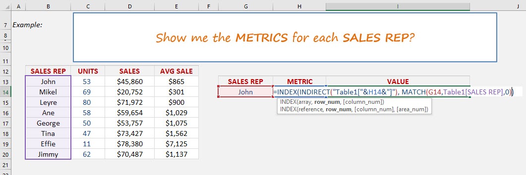
We can use the INDEX-MATCH formula and combine it with Data Validation drop down menus to return a value based on 2 criteria. This is a little advanced so you will need to drop what you are doing and really focus.  Let’s go…

Key Takeaways

• Combine INDEX & MATCH for Powerful Lookups – Using INDEX MATCH allows more flexibility than VLOOKUP, especially when dealing with non-adjacent columns.

• Handle Multiple Criteria with Array Formulas – You can use MATCH with multiple criteria by combining conditions (e.g., using & or *) to find an exact row that meets both criteria.

• Integrate Data Validation for Dynamic Inputs – Adding Data Validation dropdown lists lets users select criteria dynamically, ensuring clean and controlled inputs for the lookup.

• Avoid VLOOKUP Limitations – INDEX MATCH works both left-to-right and right-to-left, and doesn’t require the lookup column to be on the left side like VLOOKUP.

• Efficient and Scalable Solution – This method is faster, more reliable, and easier to maintain, especially when dealing with large datasets or changing table structures.

Quick Overview

What does it do?

Searches the row position of a value/text in one column (using the MATCH function) and returns the value/text in the same row position from another column to the left or right (using the INDEX function)

Formula breakdown:

=INDEX(array, MATCH(lookup_value, lookup_array, [match_type])

What it means:

=INDEX(return the value/text, MATCH(from the row position of this value/text))

---

First we need to convert our data into an Excel Table by pressing Ctrl+T

See tutorial on how to convert to an Excel Table here

We then create drop down menus for our Sales Rep column and another one for our Units/Sales/Avg Sale column names

See tutorial on how to insert drop down menus here

Once the above are done we need to create our formula.

STEP 1:  We need to nest an INDIRECT function within the INDEX function and reference the Metric cell name (H14) with our Table name (Table1):

=INDEX(INDIRECT(“Table1[“&H14&”]”),

This will give us our dynamic column name within the Excel Table.

 

STEP 2: We need to lookup our Sales Rep within the Sales Rep column table:

=INDEX(INDIRECT(“Table1[“&H14&”]”), 

MATCH(G14,Table1[SALES REP],0))

So by combining these formulas we can choose two criteria (Sales Rep & Metric name) to return the respective value.

 

Frequently Asked Questions

What is the advantage of using INDEX MATCH over VLOOKUP?
INDEX MATCH is more flexible, allows lookups in any direction, and works well with non-adjacent columns, unlike VLOOKUP.

How do I apply multiple criteria in INDEX MATCH?
You can combine criteria within the MATCH function using an array formula, like: MATCH(1, (A2:A10=E1)*(B2:B10=F1), 0) This checks both conditions simultaneously.

Why use Data Validation with INDEX MATCH?
Data Validation creates dropdown lists so users can select valid options, reducing errors and making the lookup dynamic and user-friendly.

Do I need to use Ctrl+Shift+Enter for the formula to work?
In older Excel versions, yes. However, in Excel 365 and Excel 2019, array formulas like this work without special keystrokes.

Can I extend this method to more than two criteria?
Absolutely! Just add more conditions in the MATCH part: (Criteria1=Cell1)*(Criteria2=Cell2)*(Criteria3=Cell3)and so on, adjusting for as many criteria as needed.