The INDIRECT function mystifies lots of Excel users and one that does not get that much fan fare, but I am about to change that for you. To be totally honest, I wasn’t a big user of the INDIRECT function, but after seeing the various ways that it can be applied in to an Excel workbook, Financial Model or Excel Dashboard, I was hooked. I will take you on this series in explaining how this function works, starting from the basics and moving on to real life practical uses that will take your Excel skills to another level!
Key Takeaways:
- The INDIRECT Function in Excel is placed within the Lookup and Reference functions category, and its primary purpose is to convert text strings that represent cell references into actual cell references. This capability is especially useful when dealing with dynamically assembled references, often the case when handling data imported from external sources.
- In the realm of financial analysis, the INDIRECT function enhances productivity by allowing analysts to create dynamic cell or range references, which reduces the need to manually input cell references in formulas. This streamlining significantly speeds up the analysis process, leading to more efficient and adaptable Excel workflows.
What does it do?
Returns a reference to a range. The referenced range can be a cell, a range of cells, or a named range.
Formula breakdown:
=INDIRECT(ref_text, [a1])
What it means:
=INDIRECT(Return the referenced range, Omit if the reference is an A1 style or enter FALSE if it is a R1C1 style)
Table of Contents
Referenced Range is a Cell
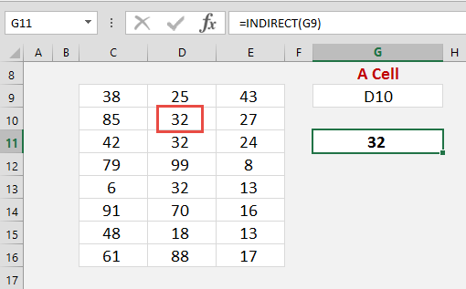
=INDIRECT(G9)
When the referenced range is a cell, the INDIRECT function will go and return the content of the referenced cell.
Say we enter in cell G9 the following A1 style: D10
In another cell we enter =INDIRECT(G9)
This will indirectly return the value that resides in cell D10, which is the number 32 in our example below:
Reference a Range of Cells
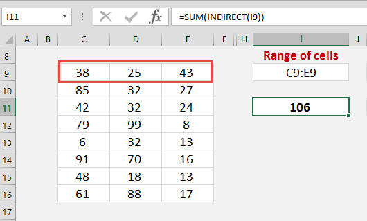
=SUM(INDIRECT(C9:E9))
When the referenced range is a range of cells, the INDIRECT function will go and return the content of the referenced cells.
We can then enter a SUM function which will total the referenced cells.
Say we enter in cell I9 the following A1 style: C9:E9
In another cell we enter =INDIRECT(I9)
This will indirectly Sum the values that reside in cells C9:E9, which is 106 in the example below:
Reference is a Named Range
=SUM(INDIRECT(NamedRange))
When the referenced range is Named Range, the INDIRECT function will go and return the content of the Named Range.
We can then enter a SUM function which will total the Named Range.
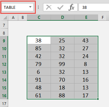
We need to create a Named Range by selecting the data range and entering a name (with no spaces) in the Name Box:
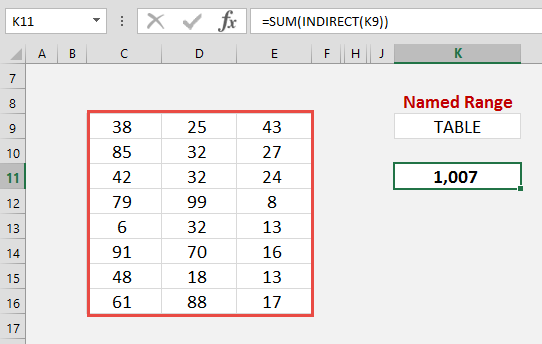
We then enter in cell K9 the following Named Range: TABLE
In another cell we enter =INDIRECT(K9)
This will indirectly Sum the values that reside in the Named Range TABLE, which is 1,007 in our example below:
Imagine having several Named Ranges that reference different data sets within a Workbook & adding a drop down menu to show the different Named Ranges.
Using this technique you can pick & choose the different data sets and with the INDIRECT function return the summation of each, thus creating an interactive Dashboard!
INDIRECT in Action Across Worksheets and Workbooks
Navigating Multi-Sheet References Smoothly
Imagine you’re working on a comprehensive project with data spread across multiple Excel sheets. For instance, you want to collate data from different departments sitting in separate sheets without rewriting formulas every time there’s a shuffle. Here’s where the INDIRECT function shines! It lets you create a dynamic reference to another sheet, using a formula like =INDIRECT($B$5&"!"&"A1"). If you place a sheet name in cell B5, INDIRECT adapts and fetches the value from A1 of that specific sheet. So, if you ever need to change to a different sheet, simply update cell B5, and you’re set—no need to alter the formula itself! See this cool example below:
External Workbook Magic: INDIRECT Beyond Boundaries
Now, extend your mastery over Excel with INDIRECT to connect not just between sheets within the same workbook but also with external workbooks. This trick feels like magic when you seamlessly extract data from entirely different Excel files. Say goodbye to the tedious task of switching between files! With INDIRECT, you can link cells across workbooks using the syntax: =INDIRECT("'[" & A2 & "]" & B2 & "'!" & C2), where A2 holds the other workbook’s name, B2 the sheet name, and C2 the cell reference. Remember to keep those external workbooks open to prevent any #REF! errors.
Savvy Integration: INDIRECT with Other Excel Functions
Pairing INDIRECT with Data Validation for Smarter Inputs
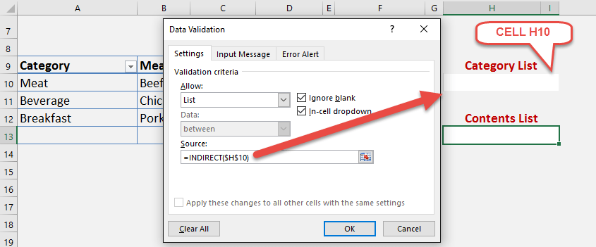
When data validation meets the INDIRECT function in Excel, you get the superpower to create dynamic dropdown menus that react to your every choice. This means as you select an option from the first dropdown list, the INDIRECT function works behind the scenes to display a corresponding set of choices in the second dropdown. This is particularly handy for creating cascading dropdown lists where your selection in one influences the options in another.
To achieve this, first ensure your dropdown items are neatly arranged in named ranges. Then, armed with a formula such as =INDIRECT(H10), where A2 is the cell with your first dropdown, Excel effortlessly updates the second dropdown list. And the beauty is, if you decide to expand your datasets or alter choices, your INDIRECT-driven dropdowns automatically adapt without extra tweaking.
Synergy with SUM, AVERAGE and More for Flexible Formulas
Expanding your Excel toolset to include INDIRECT when using functions like SUM and AVERAGE can revolutionize the way you calculate data. For example, summing values across different sheets becomes a breeze. An INDIRECT-SUM combo lets you reference cells dynamically, such as =SUM(INDIRECT("'"&A3&"'!B1:B5")), adding up the range B1:B5 from the sheet named in A3.
What’s more, you can use AVERAGE, COUNT, MAX, or any other aggregation function in a similar way. This setup is not only efficient but also flexible—when your data sources change locations or when you’re building models that require dynamic range selection, the INDIRECT function keeps your formulas adaptable and relevant.
Sidestepping Pitfalls: Troubleshooting Common Issues
Avoiding Circular References and INDIRECT Errors
To sail smoothly in Excel, you must watch out for circular references, which happen when a formula refers to its own cell either directly or through a chain of references. This can lead to incorrect calculations or Excel refusing to calculate at all. When using INDIRECT, it’s crucial to ensure that your formulas aren’t accidentally self-referencing.
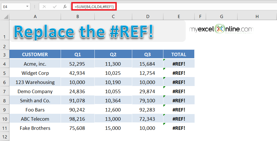
Also, you want to steer clear of other common INDIRECT errors. When you see #REF!, it usually means there’s an issue with your cell references—maybe you’ve moved some cells or mistyped a reference. Check your formulas for accuracy, confirm all named ranges exist, and ensure that your text strings match your intended references. A sharp eye and thorough checks are the best defenses against these INDIRECT issues.
Tips on Maintaining Indirect Formula Legibility
Working with INDIRECT can quickly turn your spreadsheet into an enigmatic puzzle. To keep your INDIRECT formulas easily understandable, start by breaking down complex formulas into smaller, more digestible pieces. This will help not only for your own clarity but also when others need to make sense of your work.
Another pro tip is to use named ranges within your INDIRECT functions. This can transform a cryptic cell reference like INDIRECT("Sheet1!A"&B2) into the more legible INDIRECT("SalesData"&B2). Additionally, utilize comments to annotate your formulas, providing context or explaining the purpose of certain INDIRECT functions. This can greatly enhance readability for anyone reviewing your Excel masterpiece.
FAQ: Mastering INDIRECT Function Insights
What Unique Benefits Does the INDIRECT Function Offer?
INDIRECT is a flexible charmer in Excel’s function arsenal. Its unique benefit is the ability to construct cell references from text strings, enabling dynamic formulas that can adjust as your data layout changes. This makes updating spreadsheets faster and error-free—you no longer need to manually update each cell reference. Particularly handy in scenarios that require template creation or scenarios where the data structure is volatile, INDIRECT helps your spreadsheets stay resilient in the face of change.
How Can INDIRECT Function Simplify My Excel Tasks?
Think of INDIRECT as your Excel concierge, simplifying complex tasks with its ability to read and assemble references on the fly. This simplification is especially evident when managing dashboards, financial models, or data across multiple worksheets and workbooks. By setting up a single reference cell, you can change data sources throughout your entire workbook with a simple text edit, cutting down the time spent on updates. INDIRECT also empowers data validation, leading to smarter, interdependent dropdown lists, which streamline data entry and minimize errors.
What Are Some Precautions When Using INDIRECT in Excel?
While INDIRECT is powerful, it’s wise to use it judiciously. One important precaution is to be aware that INDIRECT recalculates whenever any change occurs in the workbook. This can slow down Excel’s performance, especially within large or complex files. Also, since INDIRECT relies on text strings, ensure your source data remains consistently named to avoid broken formulas. Moreover, be careful when sharing workbooks as INDIRECT won’t update references to closed external workbooks, which may lead to errors or outdated information.
Always remember to double-check INDIRECT formulas to confirm they’re referencing the intended cells or ranges—and keep backup data or use version control for peace of mind.
John Michaloudis is a former accountant and finance analyst at General Electric, a Microsoft MVP since 2020, an Amazon #1 bestselling author of 4 Microsoft Excel books and teacher of Microsoft Excel & Office over at his flagship MyExcelOnline Academy Online Course.

