Insert Blank Rows In a Pivot Table

Pivot Table reports are shown in a Compact Layout format as a default and if you have two or more Items in the Row Labels (e.g.Month & Customer), then the Pivot Table report can look very clunky. There is a cool little trick that most Excel users do not know about that adds a blank row after each item, making the Pivot Table report look more appealing.

Key Takeaways:

• Enhanced Readability: Adding blank rows between groups in a Pivot Table improves the layout, making it easier to differentiate and analyze data within distinct categories.
• Customization Options: You can customize the spacing between groups by using the PivotTable Design tab, allowing you to insert blank rows selectively for better organization.
• Efficient Group Separation: Blank rows are particularly useful for creating visual separation in reports, helping to highlight specific data sections without altering the Pivot Table’s structure.
• Preserves Data Integrity: Adding blank rows through PivotTable settings ensures that the data remains intact and unaltered, as opposed to manually inserting rows that could disrupt the table’s functionality.
• Ideal for Presentation: Blank rows make Pivot Table reports more visually appealing and presentation-ready, enhancing the professionalism of the output for meetings or client reviews.

How to insert a row in Pivot Table

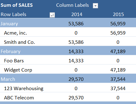
This is our starting Pivot Table:

STEP 1: Click any cell in the Pivot Table

STEP 2: Go to Design > Blank Rows

STEP 3: You will need to click on the Blank Rows button and select Insert Blank Line After Each Item

NB: For this to work you will need at least two Pivot Table Items in the Rows Labels

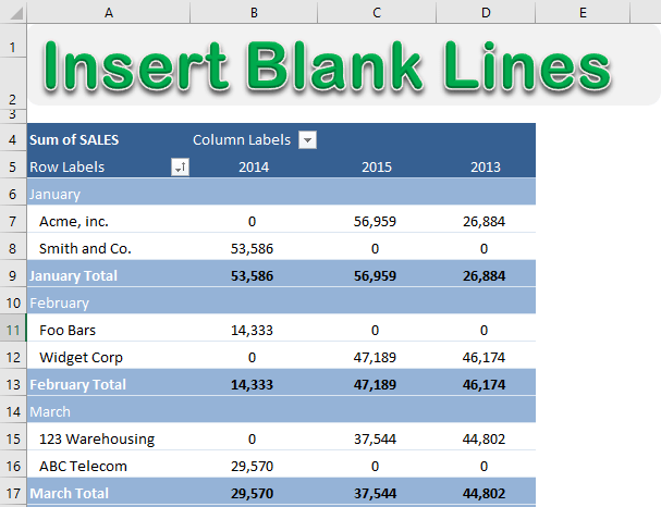
You then get the following Pivot Table report:

This tutorial shows you how to insert rows in pivot table and will make the Pivot Table look clean and more appealing.

How to remove a blank row in Pivot Table

You can easily remove this blank row from Pivot Table as well!

METHOD 1: Simply press CTRL +  Z if you have recently inserted a blank row.

METHOD 2: Go to Design > Blank Row dropdown > Select Remove Blank Line After Each Item.

This will remove the blank rows after each item!

Using the Design Tab, you can easily insert blank row in pivot table or remove it!

Frequently Asked Questions

How do I insert blank rows in a Pivot Table?

To insert blank rows, click anywhere in the Pivot Table, go to the Design tab on the Ribbon, and click Report Layout. From the dropdown, select Insert Blank Line After Each Item. This will add blank rows between grouped items in the table.

Can I remove blank rows after inserting them?

Yes, you can remove blank rows by revisiting the Report Layout in the Design tab and deselecting Insert Blank Line After Each Item. The Pivot Table will return to its original compact format.

Do blank rows affect Pivot Table functionality?

No, blank rows added through the Design tab do not affect the functionality of the Pivot Table. They are purely for visual enhancement and do not interfere with filtering, sorting, or calculations.

Can I add blank rows only to specific sections of the Pivot Table?

No, the Insert Blank Line After Each Item option applies to all grouped items in the Pivot Table. To add blank rows selectively, you would need to manually adjust the layout outside of the Pivot Table.

Why are blank rows helpful in a Pivot Table?

Blank rows improve readability by visually separating grouped data. This is especially useful in large tables or reports where distinct categories or groups need to stand out for better data interpretation and presentation.