How to Insert Hyperlink in Excel – Step by Step Guide

Hyperlinks in Microsoft Excel stand as the digital bridges that connect your data to the wider world, whether that be within the same workbook, to an external document, or to the vast expanses of the internet. These links transform static sheets into interactive maps of information, guiding users through your data with ease and efficiency.

Key Takeaways:

• Hyperlink in Excel can direct users to different sheets within the workbook, external files, web pages, or email addresses, making your spreadsheets interactive.
• Creating a hyperlink is straightforward: simply use the “Insert” menu or the HYPERLINK function to link to your desired destination.
• The HYPERLINK function allows for dynamic link creation, letting you automate hyperlink generation based on cell content.
• You can craft email hyperlinks that open your email client directly from Excel, facilitating quick and seamless communication.
• Managing hyperlinks involves both the creation and maintenance of links, including editing, testing for correct destinations, and removing unnecessary hyperlinks to keep your workbook tidy and functional.

 

Introduction to Hyperlinks in Excel

Unleashing the Power of Connectivity

Hyperlinks in Excel are more than just groovy underlined text in a color scheme that screams “click me!” They are the essential connectors in your data that bridge to other parts of your workbook, documents, email addresses, or even websites. As you’re cozying up to the idea of interconnecting your data world, let’s make sure those genius moments of yours get the execution they merit with hyperlinks.

Understanding the Basics Before You Begin

Before you start sprinkling your spreadsheet with hyperlinks, it’s essential to grasp the basics. Hyperlinks in Excel serve a simple purpose: to take you from Point A to Point B. Point B could be a different sheet in the workbook, an external file, a web page, or an email address. The power lies in their ability to make your spreadsheets dynamic and interactive. Keep in mind, the path or URL you link to must be accurate, or your hyperlink will lead to an error message—so double-check those destinations!

 

Inserting Hyperlinks Step by Step

Navigating the Insert Menu for Hyperlinks

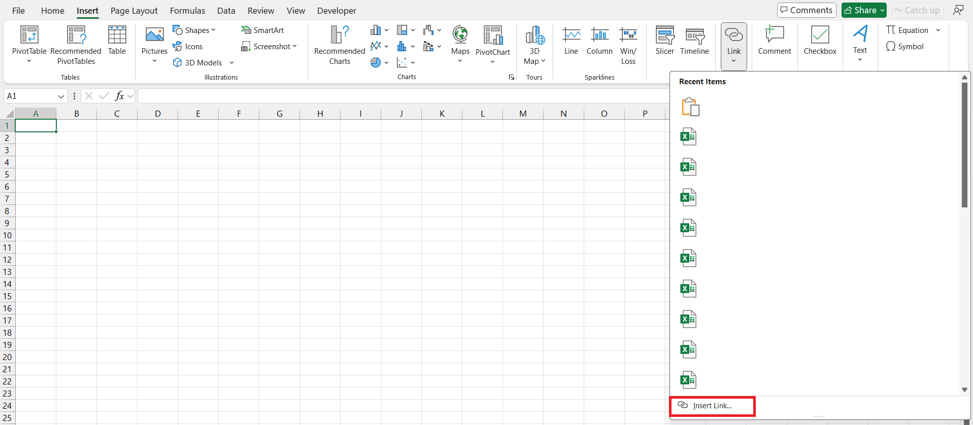
Adding a hyperlink in Excel is a walk in the park. Begin by selecting the cell where you want the magic to happen—this is where your journey starts. Then, take a gentle leap to the “Insert” tab, which is like the grand central station for all things insertion. In this bustling hub, you’ll find the “Hyperlink” option in the “Links” group.

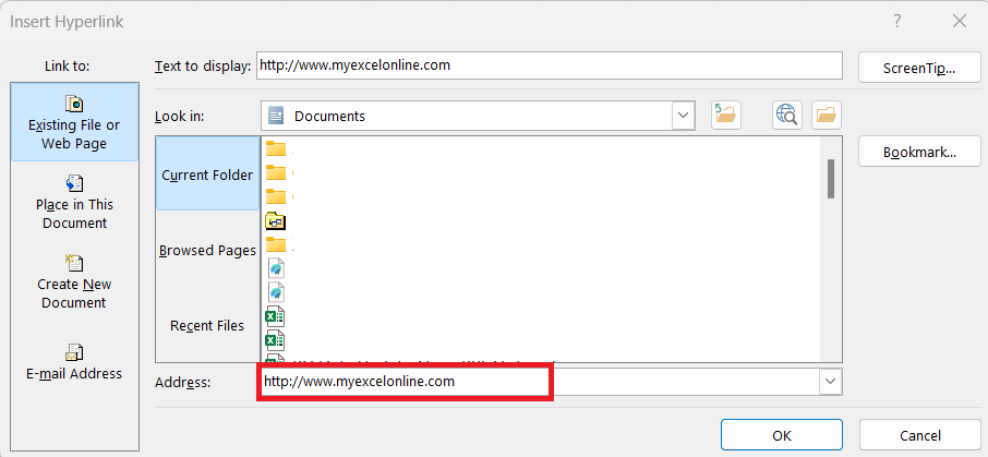
Here, a dialog box will pop up, as if to say, “Where to today?” Simply enter your desired destination in the form of a URL, a file path, or an email address and click “OK.” Voilà!

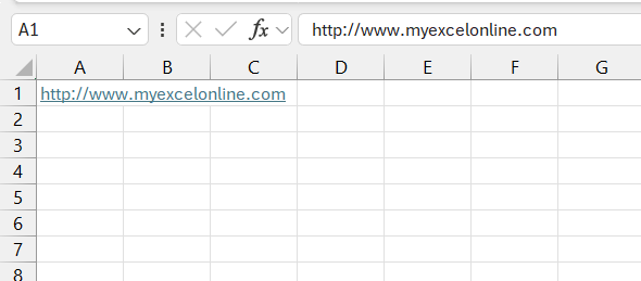
Your cell will now show blue underlined text, ready to take you to another page when clicked.

Remember, folks, always give your hyperlinks a test run to ensure they’re pointing in the right direction. You wouldn’t want to board the wrong train, would you?

Using the HYPERLINK Function Like a Pro

Mastering the art of hyperlink creation in Excel doesn’t stop at the Insert menu; there’s a nifty formula to write that deserves your attention—the HYPERLINK function. When you want to go beyond the basics and automate the process, this is your go-to tool. Its formula might seem like a mysterious incantation at first, but once you understand it, you’ll be creating links with the speed and precision of a spreadsheet sorcerer.

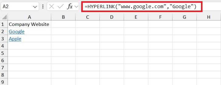
Try the formula on for size: =HYPERLINK(“http://www.example.com”, “Go to Example.com”). In this formula, the first argument is the link destination, while the second is the text that’ll appear in your cell, inviting users to click. You can link to a slew of places—online docs, different parts of your workbook, and more.

When you aim to link your Excel data to the vast expanse of the internet, a seamless connection to web pages is a must. Whether you’re crafting a directory or just want quick access to related online resources, hyperlinks serve you well. To connect a cell to a web page, click on the cell and hit the hyperlink option or use the =HYPERLINK function, as previously discussed. Once your web address (URL) is in place, you create a portal right in your spreadsheet.

Your hyperlinks can turn a static inventory list into an interactive catalog, with each item leading to its online listing, or transform a financial report by linking directly to the market data. The possibilities? Endless!

Imagine clicking a cell and being whisked away to a website where additional data and resources await. That’s some high-level spreadsheet game you’re playing.

Linking Different Sheets Within Your Workbook

Creating a well-organized and navigable workbook is like crafting a map for a treasure hunt, with each hyperlink acting as a signpost guiding the way. If your Excel workbook is expansive, containing numerous sheets, you’ll appreciate the convenience of internal hyperlinks. They’re like secret passages that instantly transport you from one worksheet to another.

Here’s how you create these navigational wonders:

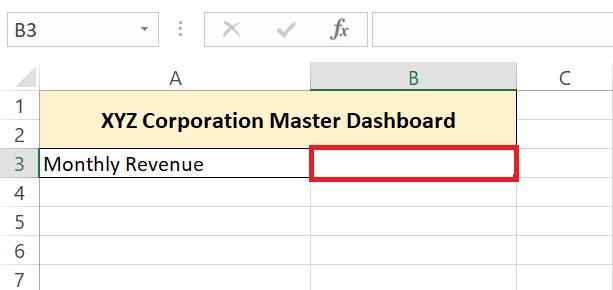
STEP 1: Select the cell where you want your hyperlink to live.

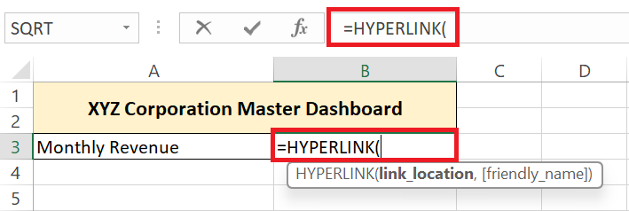
STEP 2: Enter the =HYPERLINK( to initiate the hyperlink function.

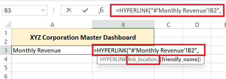
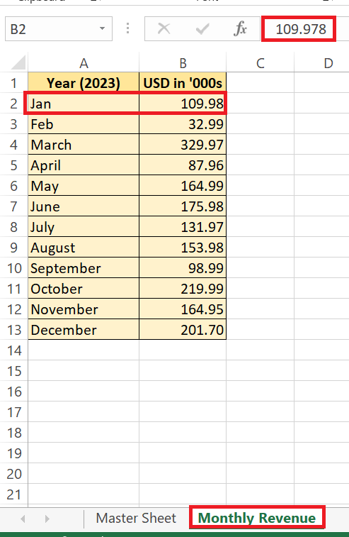
STEP 3: Specify Link Location by entering the link address within double quotes, like “#’SheetName’!Cell Reference” here in the example it will be “#’Monthly Revenue’!B2”

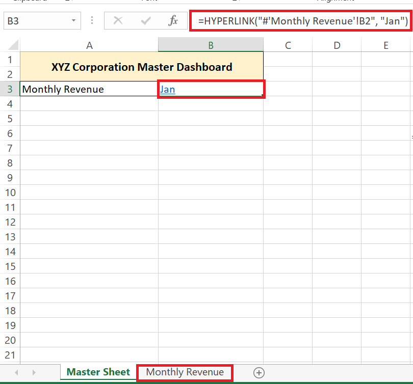
STEP 4: Specify “Friendly Name” by entering the text you want to give to the hyperlink here in the example for January Sales the text to be displayed will be “Jan”. Close the formula with a closing parenthesis “)” and press Enter.

The cell now contains a clickable hyperlink to the specified cell in another sheet.

RESULT: After clicking the hyperlink it takes you to the Monthly Revenue Sheet for January denoted by Cell B2

Now, users can hop to different sheets stress-free, while your workbook remains as neat as a pin. It’s like turning your Excel file into a choose-your-own-adventure book—each link a new chapter!

 

Advanced Hyperlink Usage

Dynamic Hyperlinks with Excel Functions

Giving life to your hyperlinks can be achieved by combining them with Excel’s powerful functions, crafting dynamic pathways that respond to your data in real-time. Ever wanted a hyperlink that updates itself when certain conditions are met? It’s possible! For instance, pair the HYPERLINK function with a VLOOKUP, and your link destination can change based on the value found.

Let’s say you have a list of company with its website details. With =HYPERLINK(VLOOKUP(A2, Sheet List, 2, FALSE), "Website Link"), Cell B2’s content determines which company detail sheet you’re zipped off to when clicking “Website Link.”

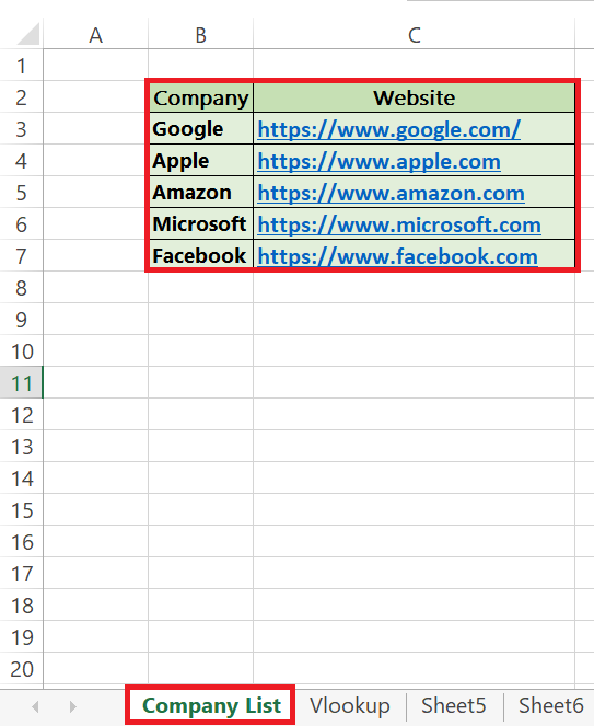
STEP 1: Organize your data with two sheets: one for the main list i.e., “Company List” and another for details. Include company names in one column and corresponding website URLs in another.

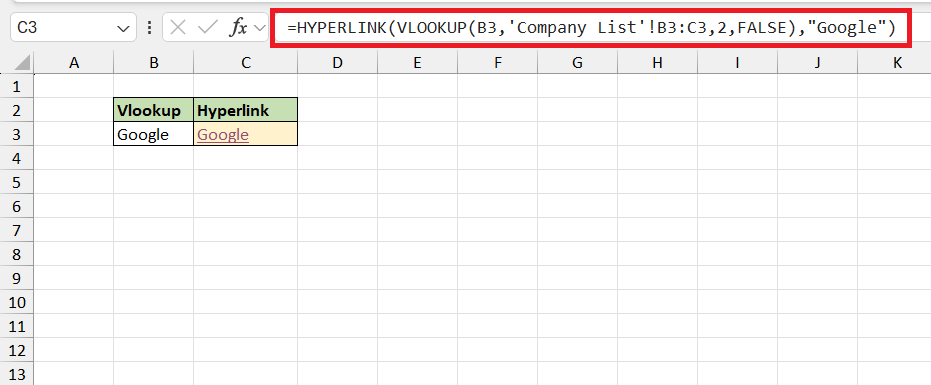
STEP 2: In the cell where you want the hyperlink in another sheet “Vlookup”, enter =HYPERLINK(VLOOKUP(B3,’Company List’!B3:C3,2,FALSE),”Google”)

The first argument of HYPERLINK is the link location. In this case, it’s the result of the VLOOKUP function, which should be a URL.

The second argument, “Google”, is the text to display in the cell. Instead of showing the URL, the cell will display the word “Google”, and clicking on it will take the user to the URL returned by the VLOOKUP function.

Dynamic hyperlinks keep adapting, saving you time and ensuring your workbook stays super interactive and user-friendly.

Craft Email Addresses that Automatically Open Outlook

Excel also facilitates smooth communication by allowing you to craft hyperlinks that, with one click, automatically open your email client, such as Outlook, to compose a message. To set this up, you’ll utilize a special ‘mailto’ protocol within the hyperlink.

Here’s the scoop on how they work:

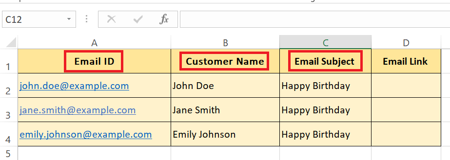
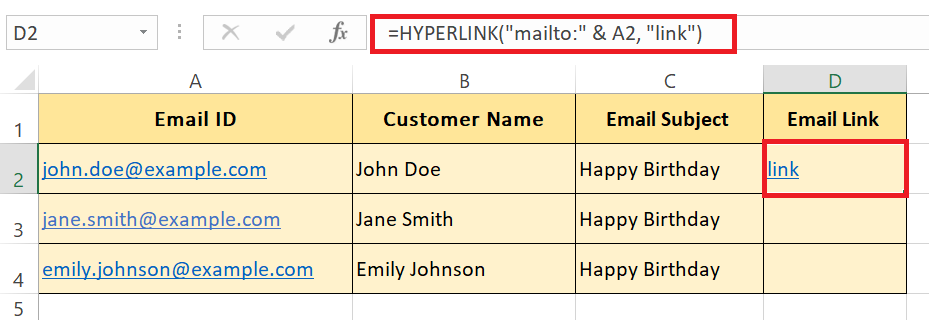
STEP 1: Arrange your data with email addresses in one column and corresponding names or identifiers in another.

STEP 2: In the cell where you want the hyperlink, use the formula =HYPERLINK(“mailto:” & A2, “Link”), where ‘A2’ contains the email address.

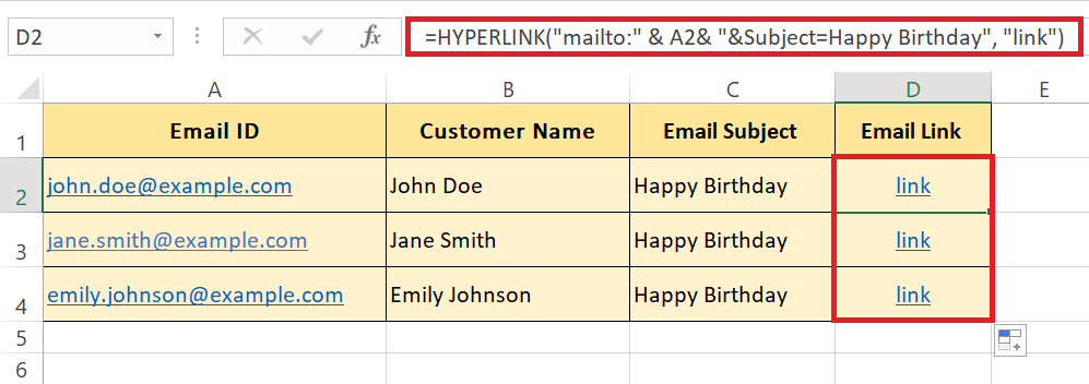
STEP 3: Customize the email subject and body by appending `?subject=YourSubject` to the email address within the formula like in the example =HYPERLINK(“mailto:” & A2& “&Subject=Happy Birthday”, “link”)

STEP 4: Drag down the formula to apply it to other rows, allowing you to compose emails with one click.

STEP 5: Click on the click to see the desired result.

Every time you click that hyperlink, your default email application revs to life, crafting a new message to the specified address, subject line at the ready. It’s as if you’ve got your own Excel-based email assistant!

Customizing and Managing Your Links

Keeping your Workbook Tidy: Removing Hyperlinks Simplified

Untangling your Excel workbook from a web of unnecessary hyperlinks doesn’t have to be a chore. To keep your digital space decluttered and your data looking sharp, Excel offers super-simple ways to remove hyperlinks.

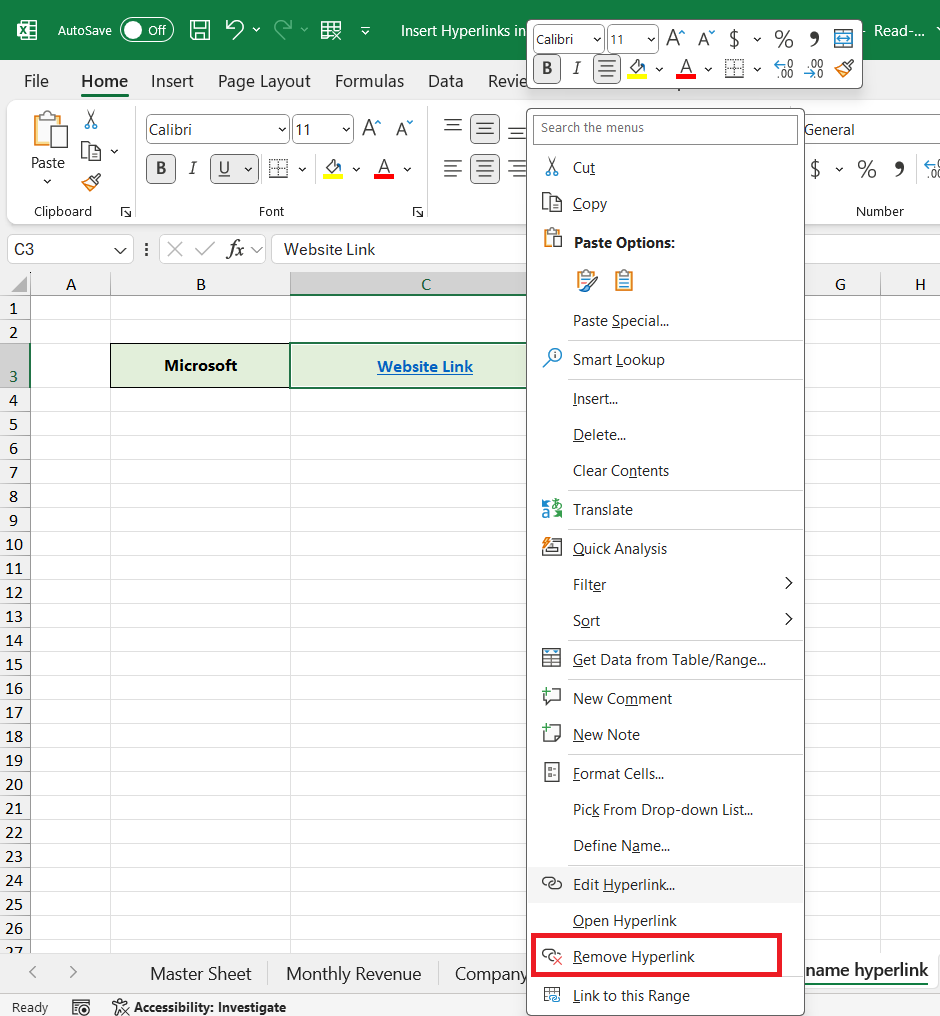
Method 1: Using the Right-click Context Menu

• Select the cell(s) wrapped in hyperlinks you want to untie.
• Tap into the context menu by a right-click.
• Hover over “Hyperlink” and lock onto “Remove Hyperlink.”

Method 2: Keyboard Shortcut Superhero

• Call the cell(s) to action by selecting them.
• Unleash the keyboard shortcut: “Ctrl + Shift + F9.”

Both methods ensure your text stays put while stripping away the hyperlinks’ clickability, banishing unwanted portals without a trace, and maintaining the pristine look of your content.

Feel like cleaning up in bulk? Excel’s got your back! To wipe away a multitude of hyperlinks in one fell swoop, simply select a larger range or your entire sheet, and bid those hyperlinks farewell using the same techniques. Ah, the joy of a tidy workbook!

 

How to Rename a Hyperlink in Excel

If the text of the hyperlink displays a file name that does not match the real file name, the hyperlink will not function. To resolve this issue, create a hyperlink to the file after it has been renamed.

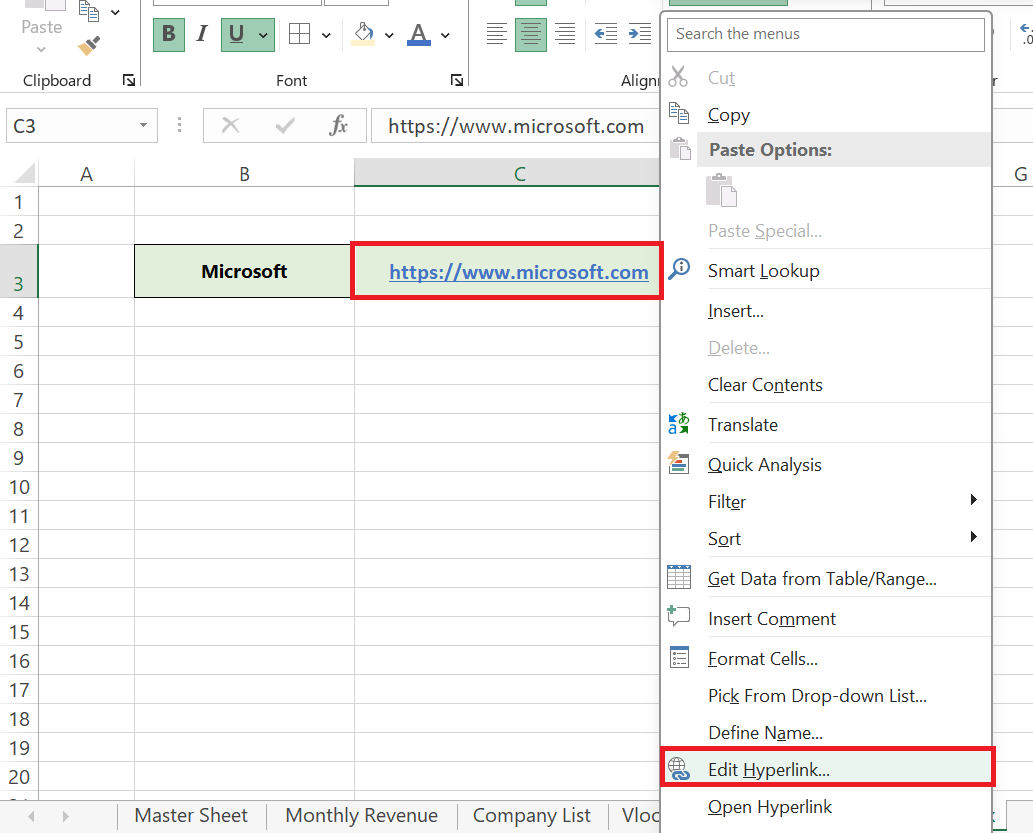
Ensure that the links in the Excel file are updated and point to the renamed file. For this, right-click the hyperlink and select ‘Edit Hyperlink’. In the hyperlink address, replace the current filename with the renamed one in the hyperlink address.

Here are the detailed steps to rename a hyperlink in Excel:

STEP 1: Choose Your Target– Click on the cell with the existing hyperlink you’re looking to rename.

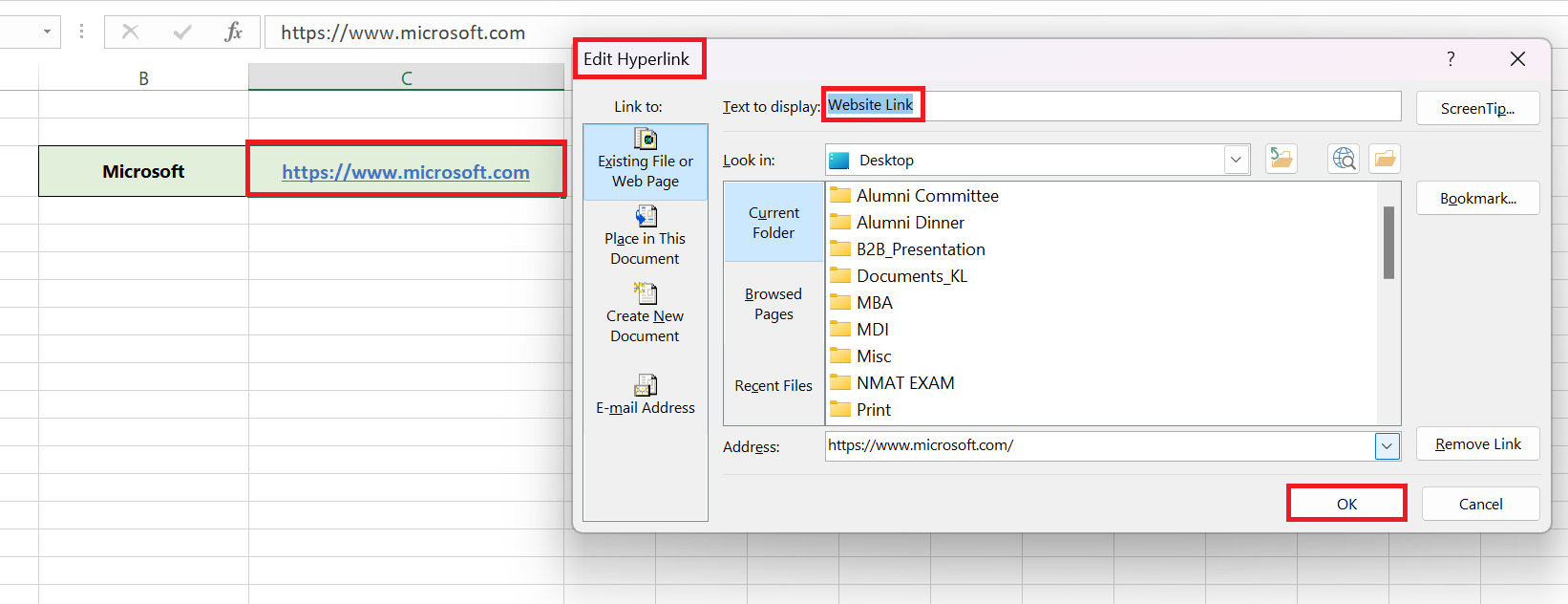
STEP 2: Dive Into the Context Menu– Right-click and select “Edit Hyperlink” from the menu.

STEP 3: Edit Hyperlink Dialog Box– Once the box pops up, it’s your cue to make your changes. Replace the outdated text with what you need, ensuring it correctly reflects the linked file’s new name. Hit “OK” to finalize the rename procedure.

Whether you’re fixing broken links due to a file rename or just updating the link text to be more descriptive, this simple maneuver ensures your hyperlinks are not just functional but also neatly labeled.

Automation with VBA for Hyperlinks

Bulk Removal of Hyperlinks with a VBA Script

Cue the orchestra, because it’s time for some more VBA wizardry! If your Excel garden has become overgrown with too many hyperlink weeds, here’s how you can remove them in bulk with a VBA script:

Sub RemoveAllHyperlinks()
Dim ws As Worksheet
Set ws = ActiveSheet
Dim i As Long
For i = ws.Hyperlinks.Count To 1 Step -1
ws.Hyperlinks(i).Delete
Next i
MsgBox "All hyperlinks removed.", vbInformation
End Sub

Follow the steps below to use VBA code to delete all hyperlinks in Excel –

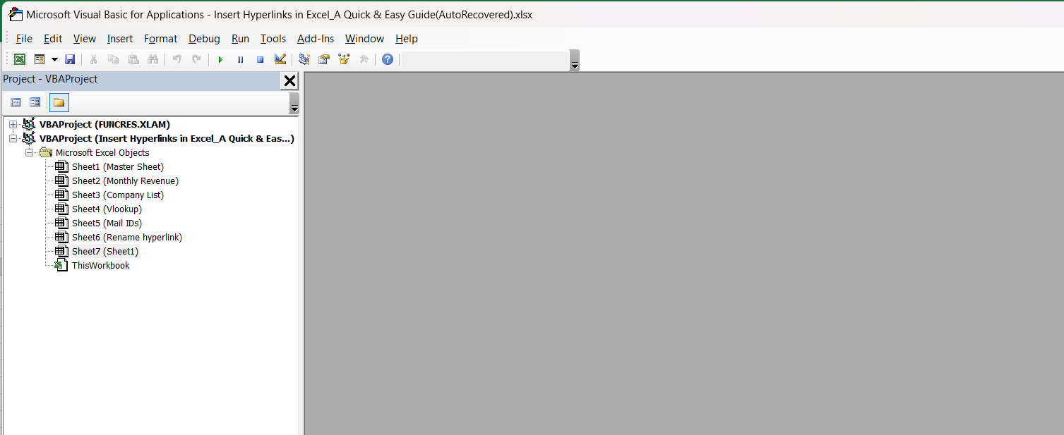
STEP 1: Access the VBA Editor: Summon the editor with Alt + F11.

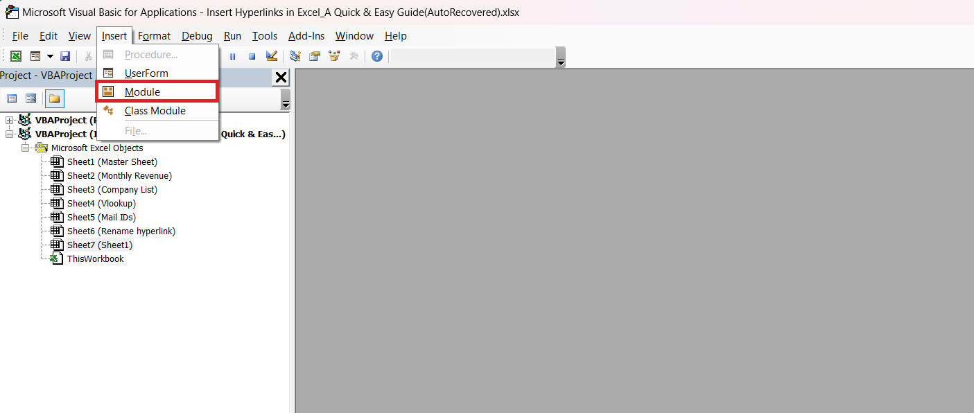
STEP 2: Introduce a New Module: Right-click on any of the workbook’s sheet names, go ‘Insert’, then ‘Module’.

STEP 3: Enchant the Module: Copy and paste the above spell, uh, script into the module window.

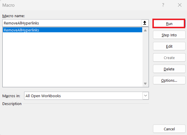
STEP 4: Activate the Macro: Close the editor, select the cells with those pesky hyperlinks, and run your macro like a digital conductor.

In a snap, your selected cells are liberated from the clutches of hyperlinks, leaving behind only the text you want to remain. This simple yet powerful VBA script is the equivalent of a one-click cleanup for your workbook’s hyperlink clutter.

It’s always wise to perform a quick rehearsal (also known as backing up your data) before the main performance to ensure nothing valuable gets lost. Happy decluttering!

FAQs About Hyperlinks in Excel

Why aren’t my hyperlinks working in Excel?

Hyperlinks may not work in Excel if they’re formatted incorrectly, pointing to a path or URL that no longer exists, or due to overprotective security settings. Ensure the destination is correct and accessible, try changing cell formats to ‘Text’, and check your security settings in the Trust Center. If hyperlinks are unresponsive, they might have been disabled by Excel’s ‘Update links on save’ option, which you can turn off in the Advanced section of Excel Options.

Can I insert a hyperlink without using the mouse?

Absolutely, you can insert hyperlinks in Excel without reaching for your mouse. Position your cursor in the desired cell and simply use the keyboard shortcut Ctrl + K (on Windows) or Command + K (on Mac) to open the ‘Insert Hyperlink‘ dialog box. From there, use the Tab key to navigate through the fields, enter the link information, and hit Enter to apply your hyperlink.

How do I remove multiple hyperlinks at once?

To remove multiple hyperlinks at once in Excel, select the range of cells containing the hyperlinks you wish to remove. Then either right-click and choose ‘Remove Hyperlinks’, or use the keyboard shortcut Ctrl + Shift + F9. This will instantly strip all the selected cells of their hyperlinks. For larger or non-adjacent selections, consider using a VBA macro for even more efficiency.

How do you convert to a hyperlink in Excel?

To convert text into a hyperlink using a mouse, first select the cell where you want to insert the hyperlink, such as cell A2. Then navigate to the ‘Insert’ tab and click on ‘Link’ in the Links group to bring up the ‘Insert Hyperlink’ dialog box. Finally, within the dialog box, choose ‘Place in This Document’, enter your desired text and cell reference, then click ‘OK’ to create the hyperlink.

What is the hyperlink function in Excel?

The HYPERLINK function in Excel is a formula that allows users to create clickable hyperlinks within a spreadsheet. Users can program these links to point to external websites, files, or different locations within the workbook by specifying a URL or file path and a display text for the link. This function is especially useful for dynamically linking large numbers of resources or for managing links through formulas.