The Ultimate Guide to Interpolation in Excel – Linear Methods Guide

When working with numerical data in Excel, I often encounter situations where I need to estimate values that fall between known data points. This process, known as interpolation, is a powerful technique for filling in missing data. In this guide, I’ll walk through how to perform interpolation in Excel using different methods, including linear interpolation and polynomial interpolation.

Key Takeaways:

• Interpolation in Excel estimates missing values between known data points, making it useful for incomplete datasets.
• Excel functions like TREND and FORECAST.LINEAR simplifies interpolation without manual calculations.
• Scatter plots with trendlines help visualize interpolated data and extract equations for further use.
• Ensuring accurate data entry and format consistency is crucial to avoid interpolation errors.

 

Introduction to Interpolation in Excel

The Basics of Interpolation

Interpolation in Excel is a fundamental data analysis technique that allows us to estimate values between two points. It’s invaluable when dealing with incomplete datasets or when needing to predict trends.

For instance, if I have different data points of a product’s sales at the beginning and end of a month, interpolation helps me estimate the sales figures for any day in between, filling in the gaps with reasonable assumptions.

Why Mastering Interpolation Matters

Mastering interpolation is crucial for making informed decisions based on incomplete or fragmented data. In fields such as engineering, finance, and science, neatly filled data sets are often a luxury. Being adept at interpolation allows us to predict and analyze trends with the data at hand, enhancing both the quality and credibility of our work.

Moreover, understanding how to interpolate correctly reduces the risk of misinterpretation, leading to more accurate projections and strategies based on the insights generated.

 

Setting the Stage for Linear Interpolation

Step 1: Enter Your Data Accurately

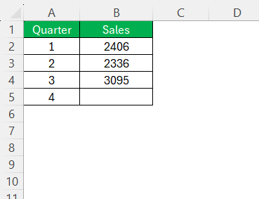
Entering your data accurately is the first and most vital step in the process of interpolation in Excel. Accurate data entry ensures the reliability of the interpolated results. Start by opening Excel and creating a new workbook. Then, input your known data points.

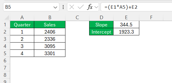
For example, if you’re looking at sales performance, you would label cell A1 as “Quarter” and cell B1 as “Sales,” followed by entering the actual data in the subsequent cells.

It’s critical to verify each entry for errors, as even a small mistake can drastically skew the interpolation outcome.

Step 2: Understand the Linear Interpolation Formula

The linear interpolation formula is the foundation for predicting values between two known data points on a linear scale. It is critical to understand that the formula derives the value of a point along a straight line drawn between two known points. The formula is expressed as y = y1 + ((x - x1) * (y2 - y1)) / (x2 - x1), where y is the estimated value, x is the interpolation point, x1 and x2 are the known x-values, and y1 and y2 are the known y-values. By grasping the logic behind this formula, we can confidently apply it to datasets in Excel to make educated interpolations.

 

Practical Methods to Perform Interpolation

Method 1: Using Basic TREND Function

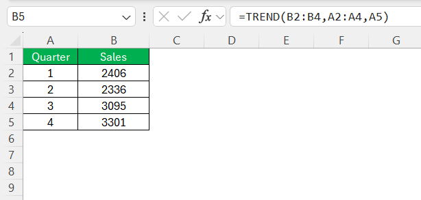
The TREND function in Excel provides a straightforward method to perform linear interpolation. To utilize it, first select the cell where you want the interpolated value to appear. For instance, to forecast sales for days that we don’t have data, enter =TREND(B2:B4, A2:A4, C2:C16), where B2:B4 are the known sales figures, A2:A4 are the corresponding days, and C2:C16 represents the range of new days for which we want the sales predictions.

Once the function is in place, simply drag the formula down through the cell range to apply it for all desired days.

Method 2: Crafting a Scatter Plot with Trendline

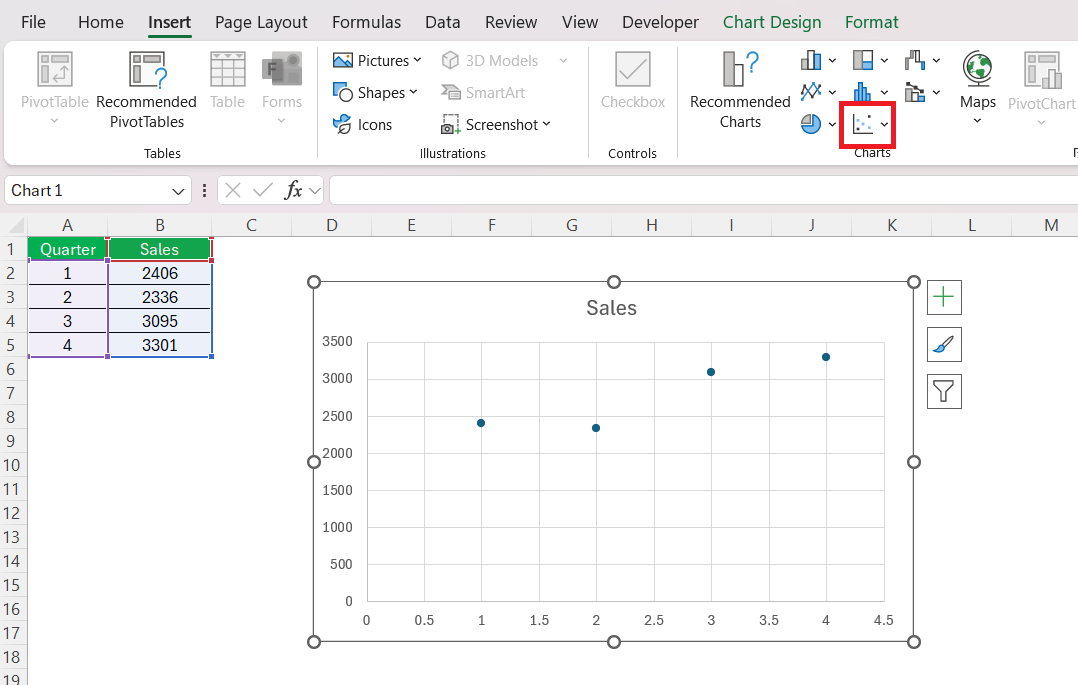
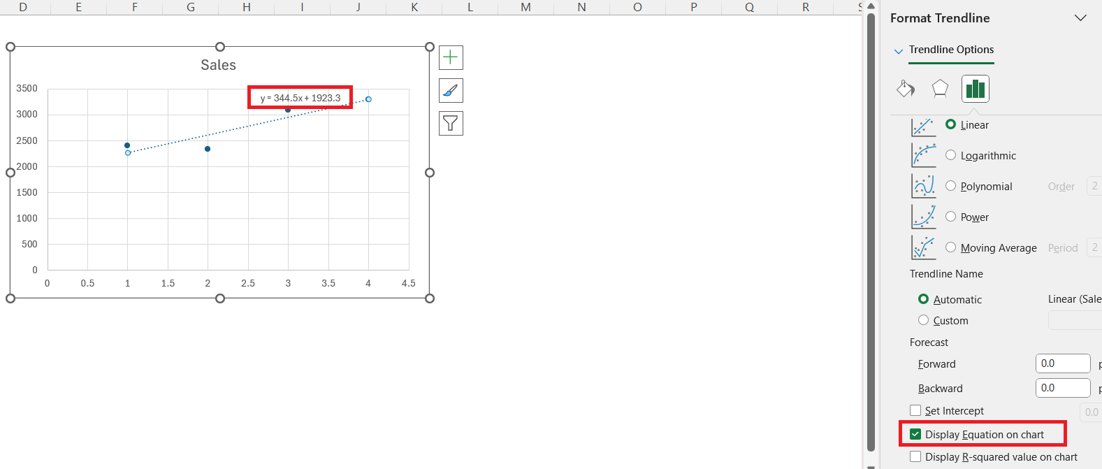
Crafting a scatter plot with a trendline in Excel is a visual approach to linear interpolation. After entering your data, highlight it and go to the Insert tab to choose a scatter plot.

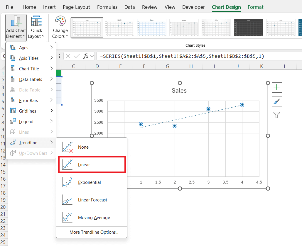
Once the plot materializes, clicking on any data point will allow access to ‘Add Chart Element’ within the Chart Design tab. From there, hover over Trendline, and select Linear.

Make sure to check the ‘Display Equation on chart’ option.

This reveals the equation of the trendline, derived from linear regression of your data, which you can use for interpolation by inserting the x-values, or independent variable, into this equation to compute the corresponding y-values or dependent variable.

 

Dive Deeper: Advanced Interpolation Techniques

Harnessing the POWER of FORECAST.LINEAR

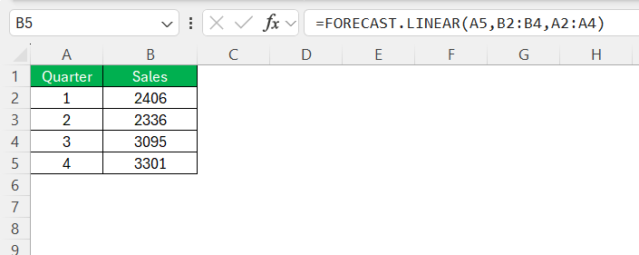
Harnessing the power of FORECAST.LINEAR can significantly enhance your ability to perform linear interpolation in Excel. This function predicts a future value along a linear trend and is an upgrade from the basic FORECAST function. Simply select a cell for the interpolated value, and input =FORECAST.LINEAR(X, known_y's, known_x's) where X represents the point you’re interpolating for, and the known_y’s and known_x’s are your existing data arrays.

FORECAST.LINEAR does the heavy lifting by calculating the y-value that corresponds to the new x-value based on the linear regression of the known data.

 

Manual Interpolation Tricks

Calculating Slope (m) and Intercept (b) Manually

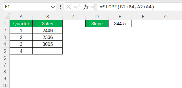
Calculating Slope (m) and Intercept (b) manually in Excel involves directly entering formulas to ascertain the parameters of the linear equation y = mx + b that best fits the given data. First, I’ll select a cell for the slope calculation and type =SLOPE(B2:B4, A2:A4), where B2 through B4 contain the dependent variable and A2 through A4 contain the independent variable. After pressing Enter, Excel calculates the slope.

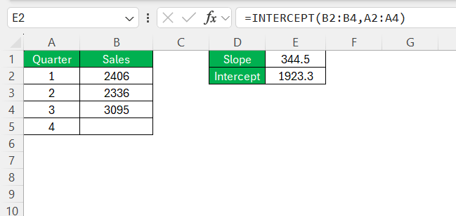
For the intercept, I’ll click on another cell and type =INTERCEPT(B2:B4, A2:A4). Once I hit Enter, Excel renders the y-intercept.

These values are crucial for manual interpolation as they determine the exact position and angle of the trend line.

Applying the Manual Interpolation Equation

Applying the manual interpolation equation in Excel requires combining the slope and intercept values with the interpolation point. Once you’ve calculated the slope (m) and intercept (b), input the x-value that you need an estimate for, which we’ll label as x_interpolated. To find the corresponding y-value (y_interpolated), input the following formula: = (m * x_interpolated) + b into a cell.

This formula takes the slope and multiplies it by your unknown x-value, then adds the intercept. The output will be the interpolated y-value, which aligns with the straight-line trend between your known data points.

 

Tips and Troubleshooting

Ensuring Data Consistency for Accurate Results

Ensuring data consistency is paramount for accurate interpolation results. Start by verifying the data type: ensure numeric data is recognized as such in Excel; dates or time values should also be formatted correctly. Consistent scales and units across the dataset are necessary; mixing different units can lead to incorrect interpolations.

Clean your data to remove duplicates, outliers, or irrelevant data points that could skew your analysis. Lastly, always perform spot-checks or use Excel’s data validation tools to keep your data consistent and thus, the interpolation results dependable.

Common Errors and How to Avoid Them

When interpolating in Excel, common errors are often due to mistaken inputs or misinterpretation of the functions used. To avoid them, ensure numeric values are used for calculations, not text that might look like numbers. Ensure that the range of x’s and y’s in your functions match and cover the entire dataset needed for the analysis.

Be mindful of Excel’s error messages such as #N/A, #DIV/0, and #VALUE, which signal problems with data sets or non-numeric inputs. Familiarize yourself with these errors and their meanings, and always review your formulae for accuracy.

 

Frequently Asked Questions

What is linear interpolation in Excel?

Linear interpolation in Excel is a method to estimate missing values that lie on a straight line between two known points. It predicts values within the range of a dataset by using the linear equation that connects the dots, enabling smoother data analysis and decision-making.

What Are the Limitations of Excel’s Interpolation Methods?

Excel’s interpolation methods are limited by the assumption of linearity between data points and cannot perfectly model curves found in more complex datasets. Additionally, they can’t interpolate outside the range of known values—this is extrapolation and involves more risks and assumptions. Always verify the appropriateness of the interpolation method for the data at hand.

Can Non-linear Data be Interpolated Using Excel?

Yes, non-linear data can be interpolated using Excel by employing methods such as polynomial or spline interpolation. These techniques cater to data that exhibit non-linear relationships. Excel doesn’t have direct functions for these, but you can use tools like the GROWTH function or leverage the flexibility of Excel’s chart tools to fit non-linear trendlines and derive equations for interpolation.

Is there an interpolation function in Excel?

There isn’t a dedicated interpolation function in Excel, but various functions like FORECAST.LINEAR, TREND, and LINEST can be utilized to perform linear interpolation. For non-linear interpolation, you may have to use more complex array formulas or leverage Excel’s graphical trendline options.

What is the formula for calculating interpolation?

The formula for calculating linear interpolation is y = y1 + ((x - x1) * (y2 - y1)) / (x2 - x1), where y is the interpolated value, x is the independent variable you’re solving for, and x1, x2, y1, y2 are the known values on either side of x. It assumes a straight-line relationship between the points.