How to Find the Largest Number in Excel Fast

When working with data in Excel, there are times when I need to quickly identify the largest number in a dataset. Whether I am analyzing sales figures, exam scores, or financial data, finding the maximum value helps me make better decisions. Thankfully, Excel offers several easy methods to achieve this.

Key Takeaways:

• The MAX function quickly identifies the highest number in a dataset while ignoring text, blanks, and logical values.
• The LARGE function allows me to find not just the highest value but also the second, third, or any nth largest value.
• Combining MAX with conditional functions like MAXIFS helps filter data and find maximum values based on specific criteria.
• Using INDEX and MATCH with LARGE enables dynamic ranking and retrieval of related information in complex datasets.
• Common issues with MAX and LARGE include non-numeric data, incorrect references, and k values larger than the dataset.

 

Unlocking Excel’s Potential: Find the Largest Number with Ease

The Essential Guide to the MAX Function

The MAX function in Excel is my go-to tool for quickly finding the highest numerical value. Whether I’m analyzing financial records, calculating statistical data, or comparing sales figures, it simplifies the process effortlessly. It automatically ignores text, logical values like TRUE and FALSE, and blank cells, ensuring accurate results. For example, if I enter =MAX(12,17,25,11,23), Excel returns 25—the highest number in the list.

This function becomes indispensable when I’m working with large datasets that require quick and precise analysis.

Unleashing the Power of the LARGE Function

The LARGE function takes my Excel data analysis to the next level, giving me a more refined way to find the largest values in a dataset. Instead of just identifying the single highest number, I use LARGE to pinpoint the second, third, or any nth largest value I need. It’s especially helpful when I want to identify the top 3 sales figures or highest scores in a dataset. The syntax is simple:

=LARGE(array, k)

• array – The range of numbers I want to evaluate.
• k – The position (rank) of the value I want to retrieve.

For example, suppose I have sales data and need to find the largest value (1st highest) and second-largest value (2nd highest) values.

The largest value (1st highest):

=LARGE(A2:J2, 1)

This returns 500, the highest value in the dataset.

The second-largest value: =LARGE(A2:J2, 2)

This returns 420, the second-highest number in the dataset.

By using the LARGE function, I can quickly rank my data without manually sorting it, making it a powerful tool for sales analysis, performance ranking, and more!

 

Deep Dive into Excel Functions for Maximum Values

Crafting Formulas: The Basics of MAX and LARGE

Understanding the fundamentals of the MAX and LARGE functions in Excel is essential for crafting effective formulas. MAX is straightforward, requiring one to simply specify the range or set of values from which to find the highest number, like =MAX(A1:J1).

On the other hand, LARGE offers additional specificity and requires two arguments: the range of values and the nth position to extract, for example, =LARGE(A1:J1, 3) for the third largest value.

It’s important to remember that while MAX returns the single highest value, LARGE affords the flexibility of targeting the second highest, third highest, and so on, which is invaluable for tiered ranking of values within a data set. By mastering both, I ensure a comprehensive ability to analyze data from multiple perspectives.

Beyond Basic: Advanced Techniques with MAX and LARGE

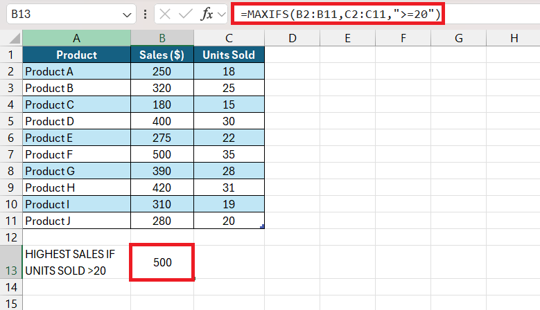
For those ready to push the boundaries of data analysis, advanced techniques with MAX and LARGE can reveal even deeper insights. By combining MAX with conditional functions like MAXIFS, I can filter and find the maximum value based on specific criteria. This is perfect for complex datasets where context matters. For instance, =MAXIFS(B2:B11, C2:C11, “>=20”), this formula looks for the highest sales figure (B2:B11) only where the corresponding “Units Sold” column (C2:C11) is 20 or more.

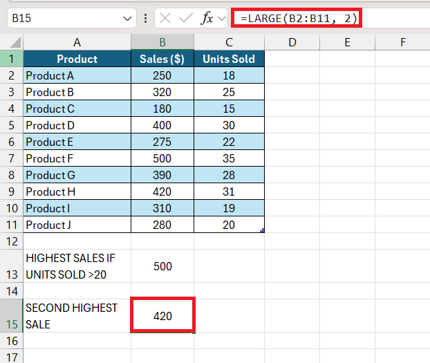
Using LARGE to Find the Second-Highest Sales Figure

This formula returns the second-largest sales figure in the dataset.

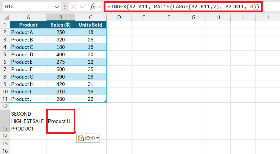
LARGE can be paired with other functions, such as INDEX and MATCH, for even more intricate data manipulation. For example, I could use =INDEX(B1:B10, MATCH(LARGE(A1:A10,2), A1:A10, 0)) to not only find the second largest value in A1:A10 but to also return a related value from another column. These techniques prove instrumental when I need a detailed and refined analysis for decision-making.

• LARGE(B2:B11,2) finds the second-highest sales value, which is 420.
• MATCH(LARGE(B2:B11,2), B2:B11, 0) looks for the position of 420 in the sales column (B2:B11) and returns its row number.
• INDEX(A2:A11, row_number) retrieves the product name from column A that corresponds to this row number.

Product H (since it has the second-highest sales of 420).

By combining these functions, I can dynamically rank values and extract related information, making my data analysis more efficient and insightful.

 

Troubleshooting Common Excel Hurdles

MAX or LARGE Not Working? Here’s Why!

When MAX or LARGE functions seem to malfunction, this typically traces back to a handful of common issues. A recurring problem is non-numeric data blended within the range, which LARGE ignores but can cause MAX to return an unexpected result if logical values or text are present. Another pitfall is incorrect cell references or selecting an array that doesn’t actually contain the data I intend to analyze.

For LARGE, specifying a k value larger than the array size is a mistake I’ve noticed – it results in an error since I’m asking Excel to find a value that simply doesn’t exist. Also, errors within the range can affect both functions – MAX will ignore them, but LARGE will return an error if the kth largest value doesn’t exist due to those errors.

Understanding these nuances is key to troubleshooting. If the functions still don’t work as intended after these checks, I look for hidden characters, and formatting issues, or even review Excel’s calculation settings.

 

FAQ: Excel’s Largest Number Conundrums Solved

What is the Difference Between MAX and LARGE in Excel?

MAX in Excel finds the highest value in a set, ignoring text and logical values. LARGE, on the other hand, allows me to specify which ‘nth’ largest value to retrieve from a dataset. While MAX returns the single largest number, LARGE gives flexibility to identify the second, third, and subsequent largest figures, useful for more detailed analyses.

How Can I Get Excel to Ignore Zeros When Finding the Max Value?

To have Excel ignore zeros when finding the max value, you can combine the MAX function with an IF statement: =MAX(IF(range<>0,range)). This formula ensures that only non-zero values are considered for the maximum value calculation. Remember to press Ctrl + Shift + Enter to make it an array formula.

Why Do I Get an Error When I Use the MAX Function?

If you’re encountering an error using the MAX function, it could be due to non-numeric values or errors within your range. MAX will return an error if it encounters any cell in the range that contains an error. Check your data for text values, logical values, or error conditions like #DIV/0! and ensure all numbers are formatted correctly.

How Can I Highlight the Largest Number in a Range or Row?

You can use Excel’s Conditional Formatting feature to highlight the largest number in a range or row. Simply select the cells, go to Home > Conditional Formatting > Top/Bottom Rules > Top 10 Items, and set it to 1. This will format the largest number distinctly. For highlighting across rows, use a formula within Conditional Formatting such as =A1=MAX($A1:$D1) and apply it to each row.

Is There a Way to Find the Max Value That Ignores Specific Errors?

Yes, to find the max value and ignore specific errors, utilize the AGGREGATE function. This function can be set to ignore errors within your data, like so: =AGGREGATE(4, 6, range). The number 4 indicates the MAX function, while 6 compels the formula to ignore errors, effectively extracting the maximum value despite any troublesome data points.