Linking Excel Tables in Power Pivot

When you have multiple tables, Power Pivot can help you link them together. After linking them together you can then create a Pivot Table that will give you a single view of data. We have a specific example for you using a Name Table and a Sales Table.

Key Takeaways:

• Establish Relationships Between Tables – Power Pivot allows you to link multiple tables using relationships, eliminating the need for VLOOKUP and improving data efficiency.
• Use a Common Key for Linking – To create a relationship, ensure that both tables have a common key, such as an ID or unique identifier, to properly connect data.
• Create Relationships in Diagram View – The Diagram View in Power Pivot provides a visual way to drag and connect tables, making it easier to manage relationships.
• Enable Efficient Data Analysis – Linking tables in Power Pivot allows you to analyze large datasets dynamically without needing to merge them into a single table.
• Use DAX for Advanced Calculations – Once tables are linked, you can use DAX (Data Analysis Expressions) to perform advanced calculations across related tables for deeper insights.

The Data Setup

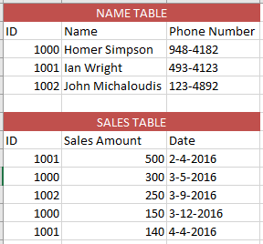
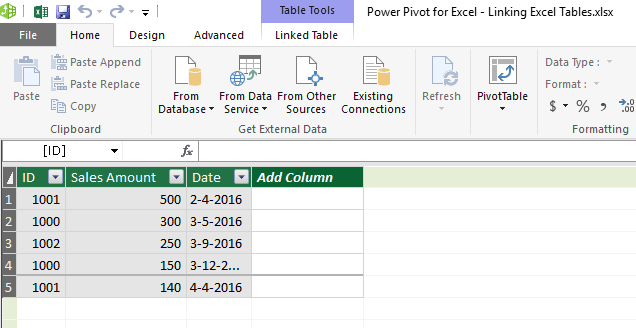
What we will focus on is a simple example of two Excel Tables: a Name Table and a Sales Table.

What we want to know is how much each Employee made in Total Sales. 

You can see that each employee is uniquely identified by the ID number, which is also used in the Sales table.

How to Link Excel Tables in Power Pivot

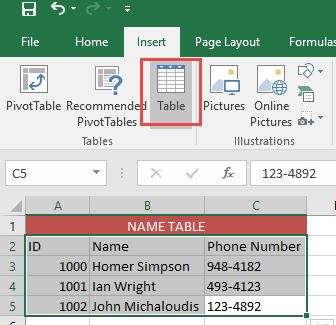
STEP 1: Select your first table. Go to Insert > Table. Click OK.

 

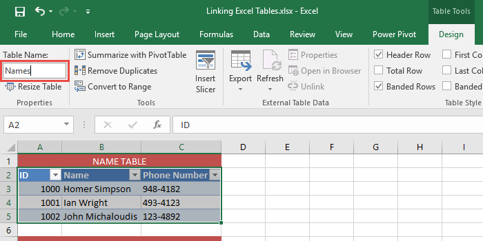
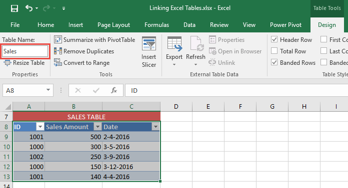
STEP 2: Go to Design > Table Name  and give your new Table a descriptive name. In our example, we will name it Names

 

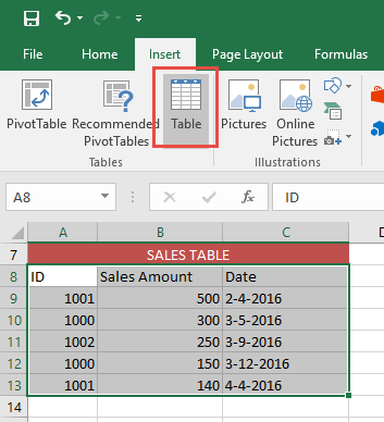
STEP 3: Select your second table. Go to Insert > Table. Click OK.

 

STEP 4: Go to Design > Table Name  and give your new Table a descriptive name. In our example, we will name it Sales

 

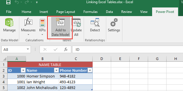
STEP 5: Select your first table. Go to Power Pivot > Add to Data Model. This will import your new Table into the Power Pivot Window.

 

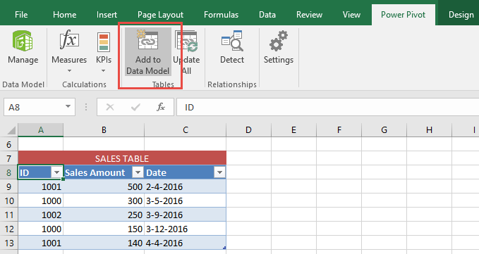
STEP 6: Select your second table. Go to Power Pivot > Add to Data Model. This will import your new Table into the Power Pivot Window.

For Excel 2010, go to PowerPivot > Create Linked Table.

 

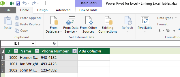
STEP 7: This will open Power Pivot Window. Your two Tables should already be loaded there.

 

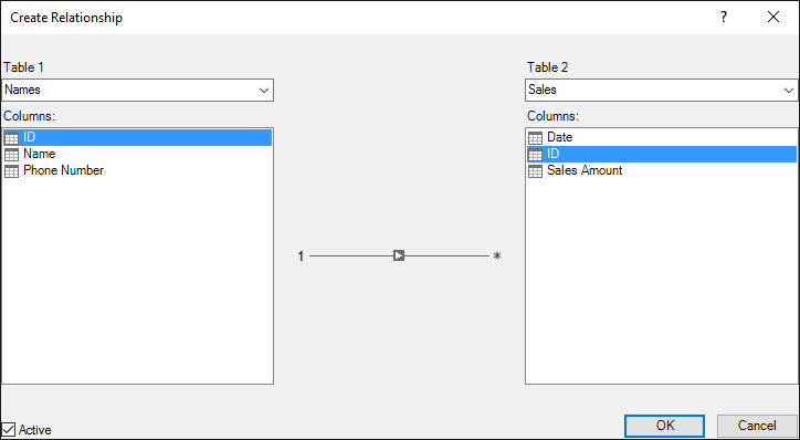
STEP 8: Go to Design > Create Relationship.

 

STEP 9: Ensure for Table 1, you set Names = ID and for Table 2, you set it to Sales = ID.

This will set the relationship and your Sales table will be able to see the values in the Names table.

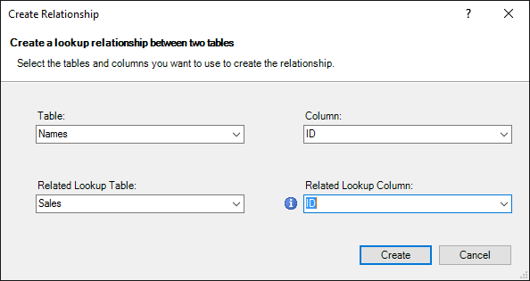
For Excel 2010, you can do the same using the Create Relationship Dialog Box:

 

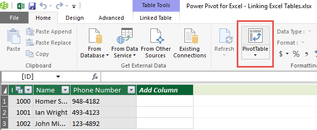
STEP 10: With this, our setup is complete.  Now it’s time to create a Pivot Table to do our analysis.

Within the PowerPivot Window, go to Home > PivotTable. 

Select New/Existing Worksheet and press OK

 

STEP 11: This will create a new Pivot Table within your Excel worksheet.

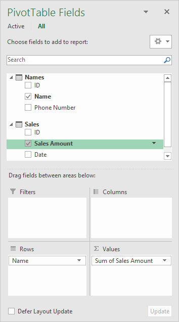
In the ROWS area put in the Name field from the Names Table,  in the VALUES area you need to put in the Sales Amount field from the Sales Table:

 

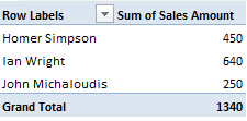
STEP 12: We now have the Names and the Total Sales Amount all in one Pivot Table.

We were able to link and consolidate two Excel Tables together with no need for VLOOKUP or helper columns…thanks to Power Pivot!

Frequently Asked Questions

How do I link two Excel tables in Power Pivot?
To link two tables, open Power Pivot, go to the Manage window, and navigate to the Diagram View. Drag and drop a common key (such as an ID column) between the tables to establish a relationship.

Why is the ‘Create Relationship’ button grayed out in Power Pivot?
The button may be grayed out if your tables are not formatted as Excel Tables (using Ctrl + T) or if you’re working with incompatible data types. Ensure both columns you want to link are of the same data type.

Can I create multiple relationships between two tables in Power Pivot?
No, Power Pivot allows only one active relationship between two tables. However, you can create multiple inactive relationships and use the USERELATIONSHIP DAX function to switch between them when needed.

What happens if I delete a relationship between linked tables?
If you delete a relationship, any calculations or PivotTables relying on that connection will return errors or incorrect results. You may need to re-establish the relationship and refresh your data.

Can I link more than two tables in Power Pivot?
Yes, you can create relationships between multiple tables, forming a data model. This allows you to build more complex reports and PivotTables without duplicating data across tables.