How to Make Loan Amortization Schedule in Excel

If you’re like me, keeping track of loans and payments can feel overwhelming without the right tools. That’s where loan amortization schedules come into play. These schedules help break down loan payments over time, showing how much goes toward interest and how much goes toward reducing the principal balance. The best part? You can easily create a loan amortization schedule in Excel.

In this article, I’ll walk you through the process of building your own loan amortization schedule in Excel. Whether you’re managing a personal loan, mortgage, or business financing, this tool will help you visualize your payments and stay on top of your finances.

Key Takeaways:

• Amortization simplifies loan management – It breaks down payments into interest and principal, helping you understand the loan payoff process.
• Excel’s formulas streamline the process – Using functions like PMT, IPMT, and PPMT makes creating a loan amortization schedule straightforward and precise.
• It helps with financial planning – Amortization schedules in Excel allow you to track payments, manage your budget, and explore refinancing options.
• Adjusting for extra payments is easy – You can account for additional payments in the schedule to see how they reduce overall interest and the loan term.
• Excel templates are a quick start – Built-in templates make it easy to create and customize loan amortization schedules based on your specific needs.

 

Introduction to Loan Amortization Schedules

Understanding Amortization in Financial Terms

Amortization might sound complicated, but as I break it down, you’ll see it’s a fundamental concept in finance that governs how a loan is paid off. In essence, amortization is the process through which a loan’s balance diminishes over time with regular payments containing portions that go towards both the principal amount and the interest incurred.

It’s the playbook that dictates the gradual reduction of debt.

Importance of Loan Amortization Schedules for Excel Users

For Excel users, grasping the importance of loan amortization schedules is paramount. These schedules serve as a financial GPS, granting us a birds-eye view of how each payment impacts the loan balance and interest over time.

They prove indispensable for personal financial management, enabling us to track our liabilities or, if we’re lenders, to manage our assets. Moreover, Excel’s powerful features afford the flexibility to tailor our schedule, aligning with specific loan agreements and our dynamic financial objectives.

 

Setting Up Your Amortization Schedule in Excel

Key Inputs for Generating Amortization Tables

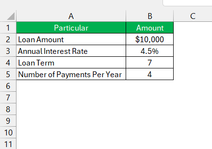
To begin crafting an amortization table in Excel, certain key inputs are essential to generate accurate calculations. These include:

• The loan amount, which is the initial principal borrowed.
• The annual interest rate, which will influence the amount of each payment going towards interest.
• The loan term in years, defining how long it will take to pay off the loan.
• The number of payments per year, which determines the frequency of payments and affects how interest accrues.

Having these inputs at your fingertips simplifies the process and lays the groundwork for a comprehensive amortization schedule.

Formulas and Functions for Amortization Mastery

Crafting the PMT Formula for Scheduled Payments

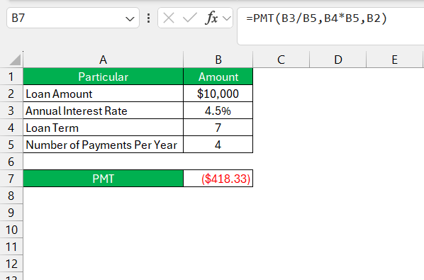
Crafting the PMT formula for scheduled payments is a pivotal step in creating an amortization schedule. The formula needs three key pieces of information: the interest rate per period, the total number of payments, and the loan amount. Here’s how to write the formula in Excel:

=PMT(rate_of_interest / number_of_payments_per_year, total_number_of_payments, loan_amount)

In our case, if we have an annual interest rate entered in cell B3, payments per year in B5, and a 7-year loan term (in B4)for a $10,000 loan in B2, we formulate it as follows:

=PMT(B3/B5,B4*B5,B2)

Remember, the result of the PMT function will be negative, representing cash outflow, but if you prefer to see it as a positive number, simply add a negative sign before the function.

Utilizing IPMT and PPMT Functions Effectively

Harnessing the power of Excel’s IPMT and PPMT functions effectively will enlighten users on the break-down of their loan payments into principal and interest components. To utilize these functions, one must understand their structure mirroring the PMT formula’s inputs but delivering different outputs.

The IPMT function computes the interest portion of a given payment. The formula has a syntax like:

=IPMT(interest_rate / num_payments_per_year, period_number, total_number_of_periods, loan_amount)

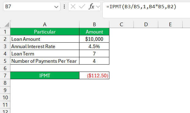
For instance, if I want to ascertain the interest component for the first payment, I might enter:

=IPMT(B3/B5,1,B4*B5,B2)

Similarly, the PPMT function reveals the principal amount paid in each payment. The formula replicates the IPMT’s syntax:

=PPMT(interest_rate / num_payments_per_year, period_number, total_number_of_periods, loan_amount)

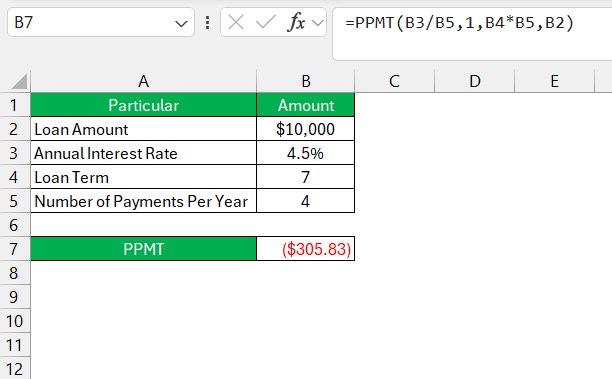
If I want to calculate the principal portion for that same payment, the formula in Excel would be:

=PPMT(B3/B5,1,B4*B5,B2)

By using these functions alongside each other, I can create a comprehensive picture of where each payment installment is going, allowing me to navigate the path of my loan’s lifecycle with clarity and precision.

 

Practical Applications of Loan Amortization Schedules

In my experience, loan amortization schedules in Excel have several practical applications that make managing finances much easier. One of the most useful aspects is being able to track how much of each payment goes toward interest versus the principal. This helps me see exactly how my debt is being reduced over time.

I also like using it for budgeting purposes. By knowing my exact monthly payment and the breakdown, I can plan ahead for the long term, whether it’s a mortgage or a personal loan. Plus, if I’m considering making extra payments, I can use the schedule to see how that would affect the total interest paid and how quickly I can pay off the loan.

Another application that’s helped me a lot is comparing different loan scenarios. By adjusting variables like the interest rate or loan term, I can instantly see how it impacts my payment plan. This has been incredibly helpful when evaluating different loan offers or refinancing options.

 

FAQs on Loan Amortization Schedules in Excel

What is amortization?

Amortization is the process of spreading out a loan into a series of fixed payments over time. Each payment includes both principal and interest, with the interest portion decreasing and the principal portion increasing over the life of the loan, until the debt is fully repaid.

How to find the loan amortization schedule in Excel?

To find a loan amortization schedule in Excel, simply go to the ‘File’ menu, choose ‘New’, and type “amortization schedule” into the search box. Excel will display a range of templates; select one that suits your needs—like one with extra payment options—and proceed by filling in your loan details.

What Is the Benefit of Creating a Loan Amortization Schedule in Excel?

The benefit of creating a loan amortization schedule in Excel is the level of control and clarity it provides over your loan repayment plan. You can visualize the trajectory of your debt, understand the impact of additional payments, and manage interest rates over the term of the loan. It’s a strategic tool that ensures accuracy in finance management.

What Excel formulas are used for loan amortization schedules?

The main formulas are PMT for calculating the scheduled payment, IPMT for the interest portion, and PPMT for the principal portion of each payment. These functions help break down loan payments and visualize repayment progress.

How do I calculate the total interest paid on a loan using an amortization schedule in Excel?

To calculate the total interest paid, sum the interest column in your amortization schedule. You can use the SUM function in Excel to add all the values in the interest column, giving you a clear picture of how much interest you’ll pay over the life of the loan.