The Ultimate Guide to Using Lookup Function in Excel

When working with large datasets in Excel, I often need to search for specific information and retrieve related data from other parts of my spreadsheet. The LOOKUP function is a simple yet powerful tool that helps me find and return values from different columns or rows. In this guide, I’ll cover what the LOOKUP function is, how to use it, and share practical examples along with tips for avoiding common errors.

Key Takeaways:

• The LOOKUP function helps me search for a value in one row or column and return a corresponding value from another.
• It’s especially useful when dealing with large datasets sorted in ascending order for approximate matches.
• There are two types of LOOKUP functions: vector form (searches a single row/column) and array form (searches multi-dimensional arrays).
• Common errors include the #N/A and #VALUE errors, often caused by unsorted data or mismatched ranges.
• For exact matches or unsorted data, using functions like VLOOKUP or XLOOKUP is more reliable.

 

Unveiling Excel’s Lookup Function

What is the LOOKUP Function?

At its core, the LOOKUP function helps me search for a specific value in one column or row, known as the lookup vector, and then return a corresponding value from another column or row, called the result vector. It’s a great tool when I need to find a match and retrieve relevant data, such as finding a product’s name by its ID number or retrieving the most recent sales data from a list.

The LOOKUP function is especially useful when my data is sorted in ascending order, as it performs an approximate match by default. If my dataset isn’t sorted, I might not get accurate results. One of the best things about LOOKUP is that it’s simple yet powerful, allowing me to search through large datasets quickly.

What Makes the Lookup Function Essential?

The Lookup function earns its essential status due to its versatility and ease of use. For us data enthusiasts, it’s a functional cornerstone in Excel, providing quick search capability across large datasets. The beauty of this function is not just in finding data but in doing so with precision, whether we seek exact matches or wish to locate the nearest value.

This utility is indispensable when dealing with financial analysis, project management, or any task that demands fast retrieval of information from extensive tables.

However, it’s important to know that the LOOKUP function doesn’t work well with unsorted data or when I need an exact match. For such cases, I use other lookup functions like VLOOKUP, XLOOKUP, or INDEX-MATCH.

 

Types of LOOKUP Functions & Syntax

The LOOKUP function comes in two main forms: Vector Form and Array Form. While I mostly use the vector form, understanding both forms is helpful in different scenarios. Let me break down their syntax and explain how they work.

Vector Form Lookups

When we talk about surfing through data using Excel’s Lookup function, the vector form is an ideal wave to catch. In essence, surfing with vector form lookups means gliding over a single row or column to find our value—no complicated maneuvers required. Within the vector form, three parameters are crucial: lookup_value, lookup_vector, and result_vector.

Here’s a simplified breakdown of the syntax: LOOKUP(lookup_value, lookup_vector, result_vector).

• lookup_value: This is the value I’m searching for.
• lookup_vector: This is the range where I want to search for my lookup value. It could be a single row or column.
• result_vector: This is optional, and it represents the range from which I want to return the corresponding value. If I don’t specify a result vector, the function will return a value from the same lookup vector.

Array Form Lookups

Diving into array form lookups is akin to plunging into a complex dataset, seeking out treasure hidden within rows and columns of data. We use the array form when our search is not limited to a single row or column but spans across a multi-dimensional grid.

The syntax shifts simply to:

LOOKUP(lookup_value, array)

• lookup_value: This is the value I’m searching for.
• array: This is a two-dimensional range where I want to search for the lookup value in the first row or column. The function returns the value from the last row or column in the array that corresponds to the lookup value.

This form looks in the first row or column of the array to find the lookup_value, providing us with a result from the corresponding position in the last row or column of the same array. Imagine you have a table where employees’ names are in the first column and their respective pay rates in the last column; an array form LOOKUP will swiftly connect these pieces of data for us.

Yet, while we’re exploring the depths, a word of caution: the array form has its limitations and quirks. It operates under the assumption that our data is sorted, and failing to heed this can lead us to incorrect results.

Additionally, as Excel innovates, there’s a gentle steer towards more advanced functions like VLOOKUP or HLOOKUP, which offer enhanced precision and functionality. We may sometimes find relics of past Excel usage in this form, serving more as a compatibility feature with older spreadsheet programs.

 

Practical Examples – Step-by-Step Guide

To really understand how the LOOKUP function works, I’ll guide you through a few practical examples that highlight its different uses. These examples will show how I can use the function to retrieve values based on different conditions.

Example 1: Looking Up a Product Name by Product ID

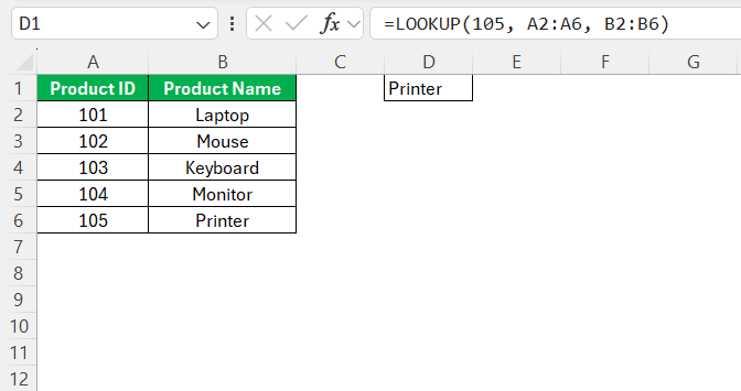
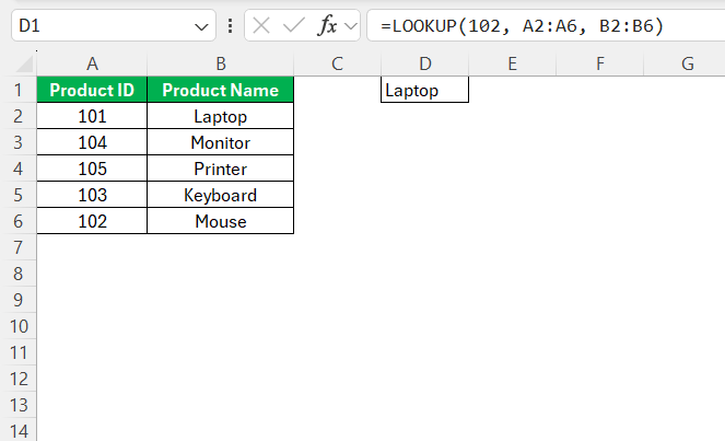
Let’s say I have a simple list of product IDs and product names in two columns. I want to find the product name for a specific product ID. Here’s how I’d use the LOOKUP function to retrieve the product name for Product ID 105:

=LOOKUP(105, A2:A6, B2:B6)

• First, I identify the lookup value (in this case, the Product ID 105).
• I then specify the lookup vector, which is the range where my Product IDs are located (A2).
• Finally, I add the result vector, which contains the Product Names (B2). This is where I’ll retrieve the corresponding product name.

The function returns “Printer” because that’s the product name that corresponds to Product ID 105.

Example 2: Returning the Last Non-Empty Value in a Column

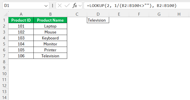
Sometimes, I need to get the last non-empty value from a column. This is particularly useful when dealing with dynamic lists that are updated frequently. Here’s how I can do it using the LOOKUP function:

=LOOKUP(2, 1/(B2:B100<>””), B2:B100)

• I set my lookup value to 2, as the LOOKUP function will search for a value in an array that is greater than 1 (since 1/TRUE results in 1).
• The formula 1/(B2:B100<>"") converts non-empty cells to 1 and empty cells to errors.
• Finally, I specify the result vector as B2:B100, where the last non-empty value will be retrieved.

This formula returns the last non-blank value from the column, which is great for keeping track of dynamic data entries.

Example 3: Using the Array Form to Retrieve Sales Data

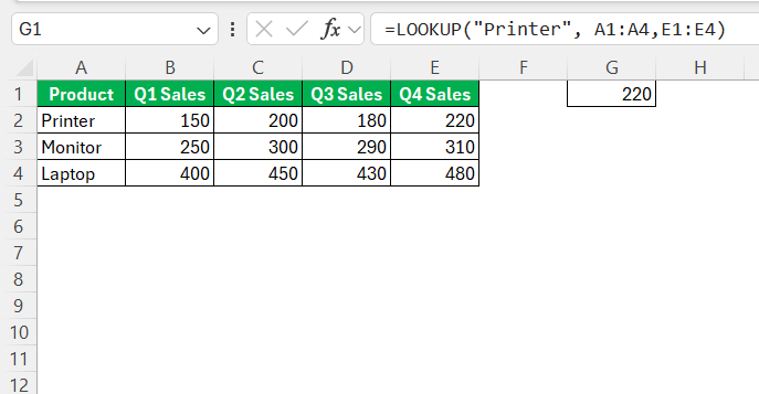
If I have quarterly sales data for multiple products, I can use the array form of the LOOKUP function to find the quarterly sales for a specific product. To find the Q4 sales for “Printer,” I’d use this formula:

=LOOKUP(“Printer”, A1:A4,E1:E4)

• I set “Printer” as my lookup value since that’s the product I’m searching for.
• I specify A1:A4 as my lookup vector, which contains the product names.
• I use E1:E4 as my result vector, where the Q4 sales figures are located.

The function returns 220, which is the Q4 sales for the Printer.

 

Common Errors and Troubleshooting

While using the LOOKUP function, I’ve run into a few common errors. Understanding these errors helps me troubleshoot quickly.

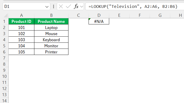
#N/A Error

This error occurs when the lookup value can’t be found in the lookup vector. It usually means that the value I’m searching for doesn’t exist in the specified range.

Double-check that the lookup value exists in the range I’ve specified. I also need to make sure the data is sorted in ascending order.

Incorrect Result

If my data isn’t sorted in ascending order, the LOOKUP function might return an incorrect or unexpected result. Since the function relies on an approximate match, unsorted data confuses the function.

Always ensure that the data in the lookup vector is sorted in ascending order.

 

FAQs

How do you use the lookup function in Excel?

To use the LOOKUP function in Excel, you begin by typing =LOOKUP( into a cell. Then, you insert the lookup_value (the value you want to search for), followed by the lookup_vector (where to find the value), and the result_vector (where to get the result from).

It could look like this: =LOOKUP(A1, A2:A100, B2:B100). This formula would search for the value in A1 within the range A2:A100 and return the corresponding value from the B2:B100 range.

How Do I Choose Between Vector and Array Forms?

Selecting between vector and array forms depends on your data’s layout and your specific needs. Use the vector form when you seek a value within a single row or column and expect a corresponding result from another single row or column. It shines for its simplicity and targeted approach.

Conversely, opt for the array form of LOOKUP if your engagement involves multi-row or multi-column arrays, and you need to find a value aligned either horizontally in the first row or vertically in the first column. Remember, this method requires sorted data to function correctly.

Can Lookup Functions Return an Approximate Match?

Absolutely, lookup functions like VLOOKUP and HLOOKUP can return an approximate match. In the final argument of these functions, input TRUE or 1 for an approximate match, particularly useful when the exact value doesn’t exist in the dataset, and you’re aiming for the next largest value that’s less than the lookup value.

Just ensure your data is sorted appropriately for this to work smoothly.

Why Is My VLOOKUP Not Producing the Correct Results?

Your VLOOKUP may return incorrect results if the lookup_value does not exactly match the data in your table_array or if the range isn’t set correctly. It’s vital to ensure that col_index_num correctly reflects the column from which you want to retrieve the data.

Also, check for any type mismatches, extra spaces, or non-printable characters, and ensure if you’re aiming for an approximate match, your first column is sorted.

What is the difference between VLOOKUP and lookup?

The difference between VLOOKUP and LOOKUP lies in their flexibility and search orientation. VLOOKUP is designed to vertically search for a value in the first column of a table array and returns a value from the same row in a specified column.

LOOKUP, meanwhile, can perform both vertical and horizontal searches, but lacks VLOOKUP’s ability to pinpoint a specific column for the return value; it works with a single row or column. VLOOKUP is typically used when you have multiple columns of related data and you need to fetch specific details based on a unique identifier.