Maximum in Excel Pivot Tables

In Excel, you can add a new column that displays the maximum in Pivot Tables in just a few clicks. And this is based on the field that you have selected. In our example, we want to show the maximum sales amount for each salesperson!

Exercise Workbook:

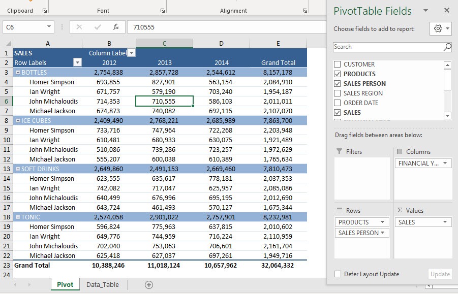
This is our Pivot Table:

STEP 1: Drag Sales to Values. This will default to become Sum of SALES

STEP 2: Click on the arrow beside Sum of SALES and select Value Field Settings

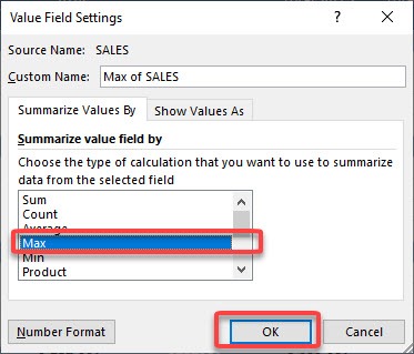
STEP 3: Select Max under Summarize value field by. Click OK

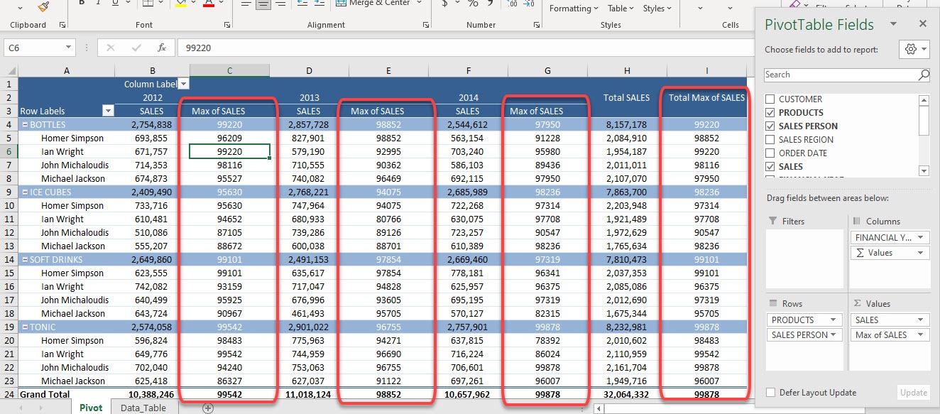
Now you have the maximum sales value for that specific year, product, and salesperson.

You can quickly check the maximum values here and determine who will get that sweet bonus!

Make sure to download our FREE PDF on the 333 Excel keyboard Shortcuts here:

Bryan

Bryan Hong is an IT Software Developer for more than 10 years and has the following certifications: Microsoft Certified Professional Developer (MCPD): Web Developer, Microsoft Certified Technology Specialist (MCTS): Windows Applications, Microsoft Certified Systems Engineer (MCSE) and Microsoft Certified Systems Administrator (MCSA).

He is also an Amazon #1 bestselling author of 4 Microsoft Excel books and a teacher of Microsoft Excel & Office at the MyExecelOnline Academy Online Course.