Multi-Select Slicer Items In Microsoft Excel Pivot Tables

We love using slicers, it just adds a level of interactivity in our reports. Did you know you can now multi-select slicer items as well?  With just a click on your slicer, you can now enable this!

Key Takeaways

• Slicers Provide Quick Filtering – Slicers allow users to filter Pivot Table data visually using buttons, making dashboards more interactive.

• Multi-Select is Built-In – Hold Ctrl (Cmd on Mac) to select multiple slicer items at once, allowing for flexible data analysis.

• Use the Multi-Select Toggle – Excel includes a multi-select icon (checkbox symbol) in the top-right corner of slicers for easy selection of multiple items.

• Instant Visual Feedback – As you select or deselect items, Pivot Tables update instantly, helping users quickly spot trends and outliers.

• Great for Dashboards – Multi-select slicers are ideal for interactive Excel dashboards, giving end-users more control over data views without altering formulas or structure.

Our Data Setup

This is our data that we will use for the Slicer.

Multi-Select Slicer Items In Microsoft Excel Pivot Tables

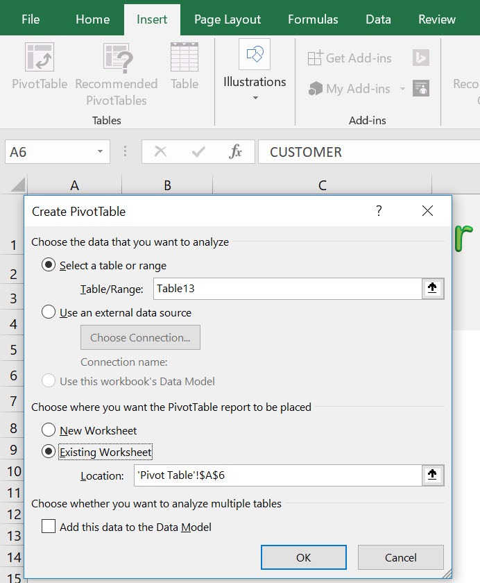
STEP 1: Insert a new Pivot table by clicking on your data and going to Insert > Pivot Table > New Worksheet or Existing Worksheet

 

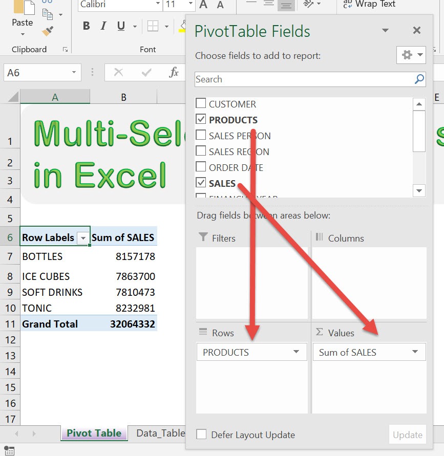
STEP 2: In the ROWS section put in the Products field.  In the VALUES section put in the Sales field.

 

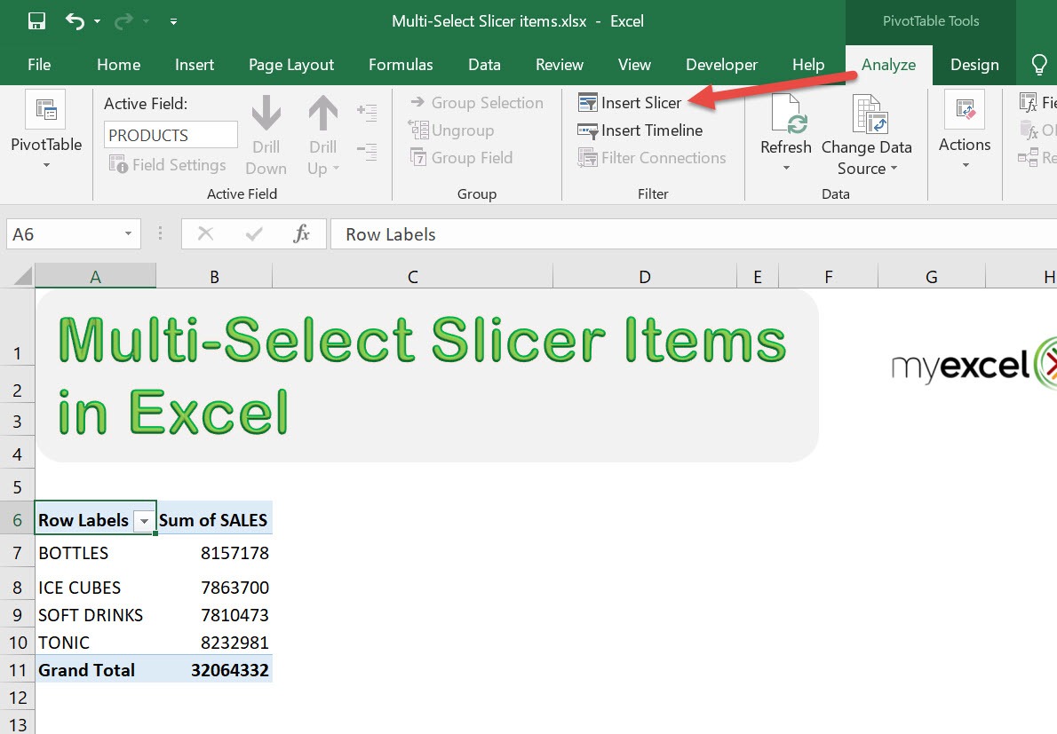
STEP 3: Let us now add our slicer! Go to PivotTable Tools> Analyze > Filter > Insert Slicer

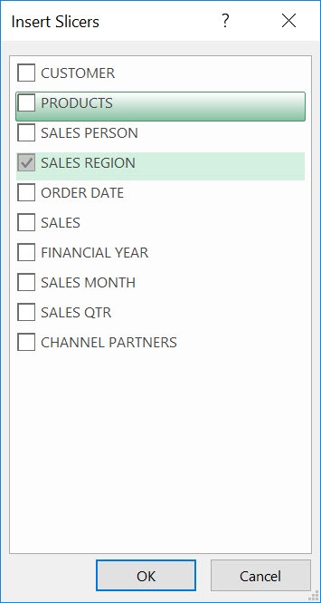
STEP 4: Make sure SALES REGION is ticked. Click OK.

 

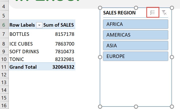
And now you have your Slicer! We just need to tick the Multi-Select button to enable this:

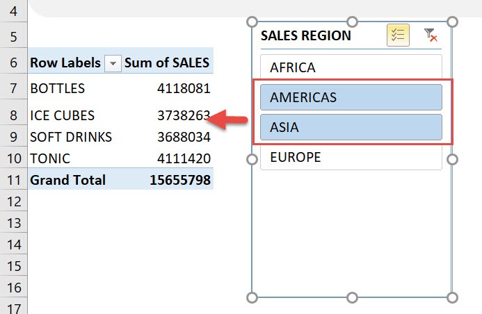
And just that, you can now multi-select slicer items! See here we have now selected Americas and Asia:

Frequently Asked Questions

How do I select multiple items in a slicer?
Simply hold the Ctrl key (Cmd on Mac) and click on each slicer item you want to select.

What does the checkmark icon on a slicer mean?
The checkmark icon enables multi-selection mode. Click it to select multiple items without using the keyboard.

Can I clear all slicer selections at once?
Yes! Click the Clear Filter icon (X in the top-right corner) of the slicer to reset all selections instantly.

Does multi-select affect multiple Pivot Tables?
Yes, if your slicer is connected to multiple Pivot Tables, multi-select will apply the same filter to all of them.

Can I customize the look of slicers for better visibility?
Absolutely! You can resize, change colors, and format slicer buttons to match your Excel report or dashboard design.