When working in Excel, one of the most common operations I perform is multiplication. But have you ever wondered what symbol Excel uses for multiplication? Unlike traditional math, where we use the multiplication sign (×), Excel follows programming conventions and uses the asterisk (*) as the multiplier symbol.
In this article, I’ll walk you through how to use the multiplier symbol in Excel, common multiplication formulas, and a few advanced tips to enhance your calculations.
Key Takeaways:
- Excel uses the asterisk (*) as the multiplier symbol instead of the traditional × sign.
- Multiplication formulas can involve direct numbers (e.g., =25*4) or cell references (e.g., =A1*B1).
- Advanced multiplication functions like PRODUCT() and MMULT() help with multiplying ranges and matrices.
- Common errors include incorrect cell references, using an ‘x’ instead of *, and ignoring the order of operations.
- Parentheses ensure correct calculations, especially in complex formulas following the PEMDAS rule.
Table of Contents
Introduction to Multiplication in Excel
Excel as a Powerful Calculation Tool
Excel is an indispensable tool for countless businesses, primarily due to its robust calculation capabilities. With a myriad of functions at our disposal, Excel serves not just as a means of entry but as a powerful computational tool that facilitates a wide spectrum of accounting and finance tasks. Its utility extends from simple data entry to complex financial modeling, making it an essential application in the modern professional’s toolkit.
Identifying the Multiplier Symbol in Excel
Multiply Using the Asterisk Symbol
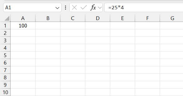
To multiply using the asterisk symbol in Excel, we merely find the symbol on the keyboard—it’s typically Shift + 8—and use it as the multiplication operator within our formulas. For instance, if I want to multiply 25 by 4, I’d enter =25*4 into a cell and press Enter, which would calculate and display the product, 100.
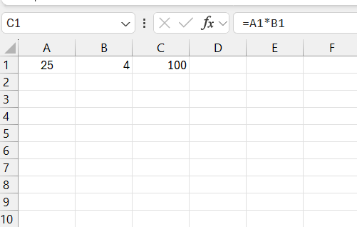
It’s that simple. Furthermore, the asterisk can combine cell references such as =A1*B1 to multiply two cell values, streamlining the process when working with data arranged in rows or columns.
Accessing Special Multiplication Functions
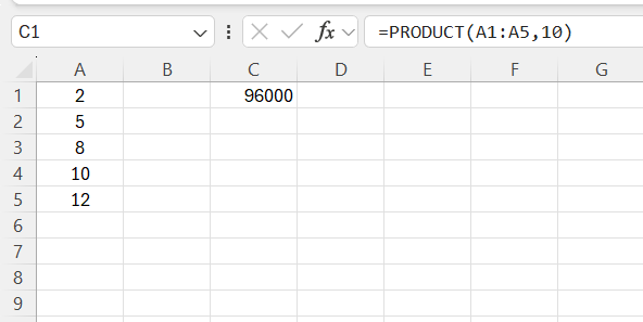
For more advanced multiplication needs, Excel presents specialized functions, such as PRODUCT() and MMULT(). The PRODUCT() function is highly versatile, enabling us to multiply numbers, cells, and ranges together. For instance, the formula =PRODUCT(A1:A5,10) multiplies all numbers in the range A1 through A5 by 10.
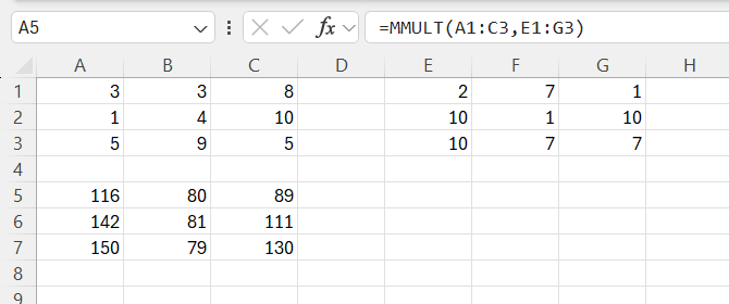
On the other hand, MMULT() allows matrix multiplication. This is particularly useful when dealing with array operations in linear algebra, and it requires the input of two arrays organized in rows and columns. The use of this function follows a specific syntax: =MMULT(array1,array2), and it’s important to note that because it deals with arrays, after typing the function, one must press “Ctrl+Shift+Enter” rather than just “Enter” to obtain the correct matrix product.
Avoiding Common Multiplication Errors
Pitfalls in Multiplying Cells and Numbers
One common pitfall when multiplying cells and numbers in Excel is inadvertently using incorrect cell references or mistyping the formula. A simple slip-up like inputting =A1*B2 instead of =A1*B1 can skew results significantly, so it’s essential to verify that all cell references are accurate.
Another mistake to watch out for is using a different symbol instead of the asterisk for multiplication. Occasionally, the use of a lower-case letter ‘x’ or a dot may seem intuitive but will result in errors. As previously stated, multiplication in Excel requires the asterisk (*) as the correct operator.
It’s also important not to forget that Excel follows the order of operations in mathematics, so when creating complex formulas involving multiple mathematical operators, using parentheses to group operations is a must to ensure calculations are performed in the correct sequence.
Correct Use of Parentheses in Complex Calculations
When constructing complex calculations that mix addition, subtraction, multiplication, and division, the correct use of parentheses is crucial to obtain accurate results. Parentheses tell Excel which operations to perform first, adhering to the PEMDAS order (Parentheses, Exponents, Multiplication and Division, Addition and Subtraction).
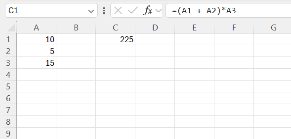
For instance, if the intention is to add two numbers together before multiplying, I might use a formula like =(A1 + A2)*A3.
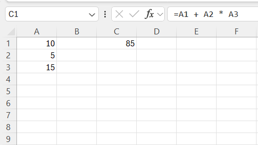
Without parentheses, the formula A1 + A2 * A3 would multiply A2 and A3 first, then add A1 to the product, which yields a different result.
Overlooking this rule can lead to costly mistakes, particularly in financial or data analysis tasks. Ensuring parentheses are strategically placed to clearly define the order in which Excel calculates parts of the formula is a fundamental skill for precise data manipulation.
Frequently Asked Questions
How to type a multiplier symbol in Excel?
To type the multiply symbol in Excel, use the asterisk (*) on your keyboard, typically accessed by holding Shift and pressing the number 8. This symbol acts as the multiplication operator when used in formulas. For example, typing =2*3 in a cell and hitting Enter will multiply 2 by 3, giving you the result of 6.
What is the Difference Between Multiplying Numbers and Multiplying Cells in Excel?
The difference between multiplying numbers and cells in Excel lies in the reference used. For numbers, you directly input values into a formula. For cells, you refer to the cell coordinates (like A1) instead of the numbers themselves. Both methods use the asterisk (*) as the multiplication operator in a formula.
Where Can I Find the Multiplication Symbol on My Keyboard?
On a standard keyboard, the multiplication symbol used in Excel, the asterisk (*), is found by pressing Shift + 8. It’s the same key used for the number 8 and enables us to perform multiplication operations in Excel and other applications.
What is the multiplier formula in Excel?
In Excel, the multiplier formula isn’t a specific function but a term generally referring to any formula that performs multiplication. It commonly involves the asterisk (*) symbol, used as the multiplication operator between numbers or cell references, such as =A1*A2. For multiplying multiple numbers or cell references, you can also use the PRODUCT function, like =PRODUCT(A1, A2, A3).
Why can’t I multiply the other cells with my constant number?
If you can’t multiply other cells by a constant number, it might be due to incorrect cell referencing. Ensure you’ve locked the constant cell reference using dollar signs (e.g., $A$1) in your formula. This makes the reference absolute, allowing the constant to be used reliably in formulas applied to multiple cells.
John Michaloudis is a former accountant and finance analyst at General Electric, a Microsoft MVP since 2020, an Amazon #1 bestselling author of 4 Microsoft Excel books and teacher of Microsoft Excel & Office over at his flagship MyExcelOnline Academy Online Course.

