New Pivot Table Features in Excel 2019 and Office 365

The best thing with Pivot Tables is that more features are getting added with Excel updates. I will give you my top 4 picks on the new Pivot Table features that can be used in Excel 2019 and Office 365:

• Personalize the Default Pivot Table Layout
• Automatic Relationship detection
• Automatic Time Grouping
• Search In The Pivot Table Fields List

Exercise Workbook:

---

Let us go over these features one by one!

Personalize the Default Pivot Table Layout

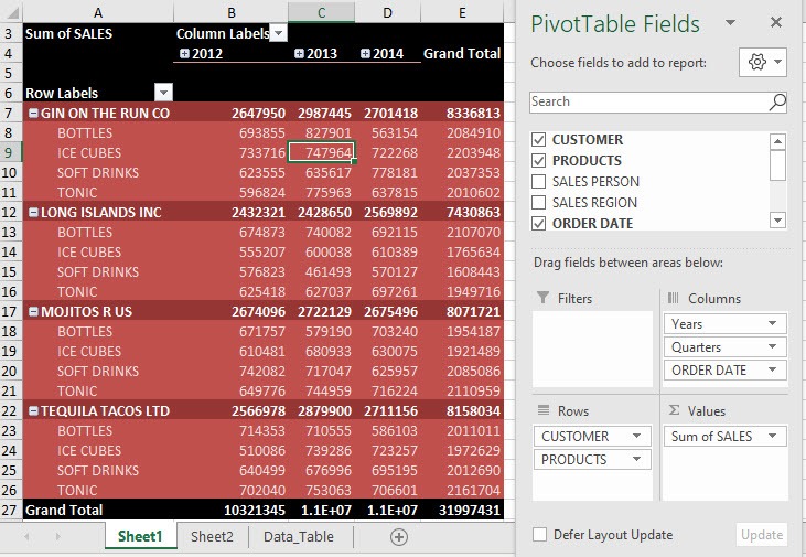
This is the default pivot table layout. The cool thing is we can make changes to this so that all future pivot tables that you create will use that same layout.

STEP 1: Go to File > Options

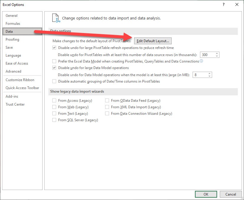
STEP 2: Select Data > Data options > Edit Default Layout

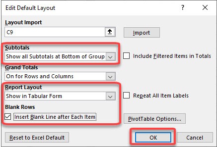
STEP 3: Let us have some fun! Try out the following:

• Subtotals – Show all Subtotals at Bottom of Group
• Report Layout – Show in Tabular Form
• Blank Rows – Tick Insert Blank Line after Each Item

You can explore more options inside PivotTable Options. Click OK.

STEP 4: Let us insert a new Pivot Table to see our new default layout!

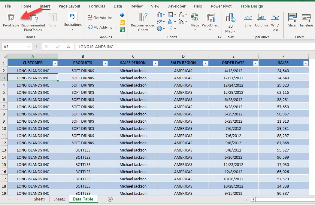
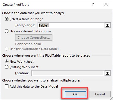
Open our data table. Go to Insert > Tables > PivotTable

STEP 5: Click OK

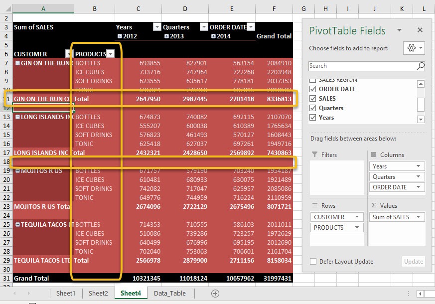
STEP 6: Setup the following:

• Columns – Order Date
• Rows – Customer, Products
• Values – Sales

And you will now see the new layout! Products column is in a separate column. The subtotals are now at the bottom of each group, and there is an empty row after each item!

 

Automatic Relationship detection

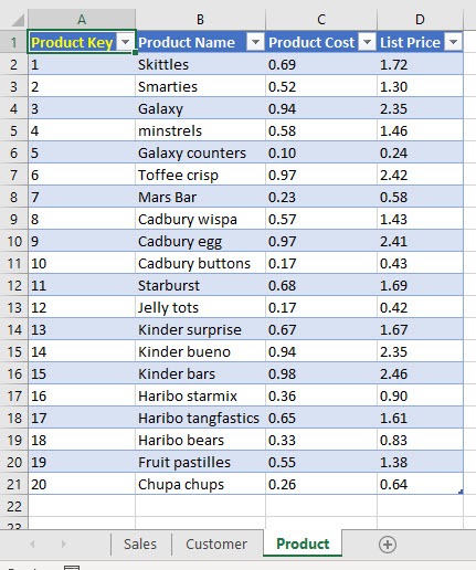
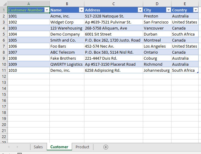
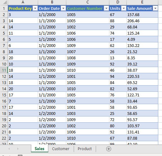
We have 3 data tables that are related to each other: Product, Customer and Sales

What connects these tables together are related columns, you will see the following:

• Product table – Product Key
• Customer table – Customer Number
• Sales table – Product Key, Customer Number

To better understand how the data model and relationships work for Pivot Tables, make sure to read this first.

STEP 1: The cool thing is once we add this to our data model, Excel is able to auto-detect the relationships when we work on the Pivot Table.

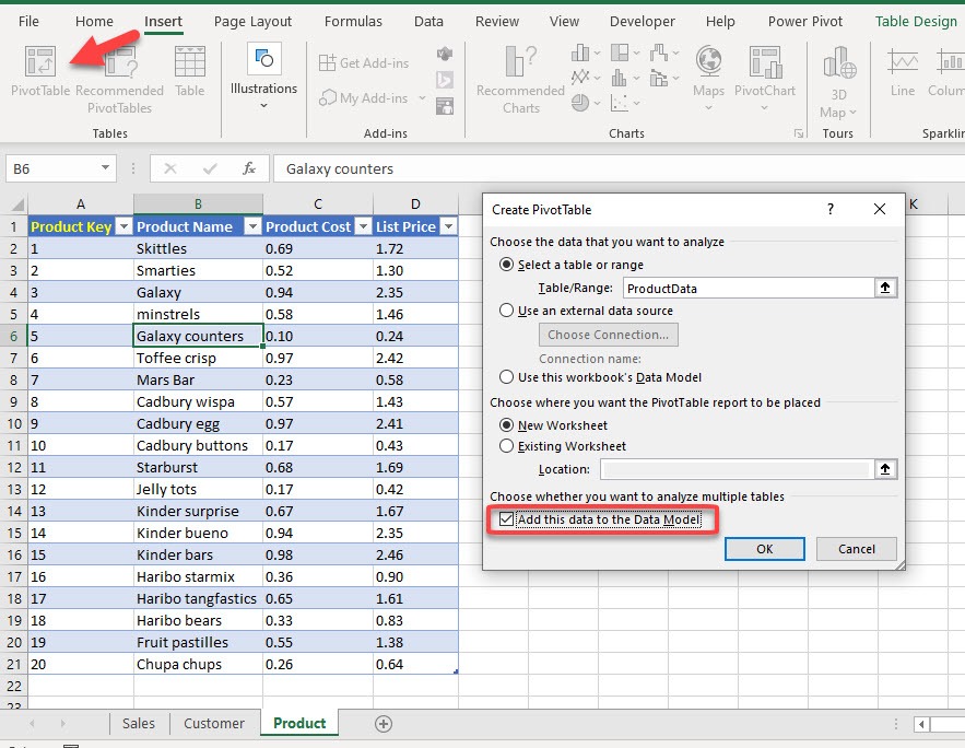
Select anywhere in one of our data tables. Go to Insert > Tables > PivotTable

Make sure Add this data to the Data Model is ticked. Click OK

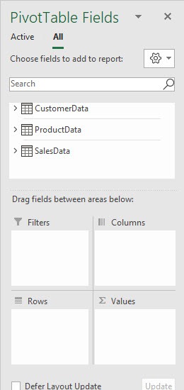
STEP 2: You will see that all of the tables are added to the data model. Select All and you will see all 3 tables are listed there.

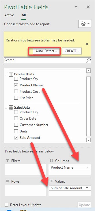
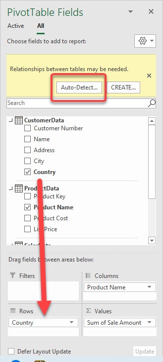
STEP 3: Let us see how Excel works its magic! Setup the following:

• Columns – Product Name
• Values – Sale Amount

Click Auto-Detect

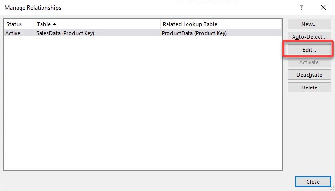
STEP 4: Select Manage Relationships to see what was created automatically

Click Edit

STEP 5: This is cool as the relationship between Sales and Product tables is correct! Excel is able to link these tables together via the Product Key columns. Click OK.

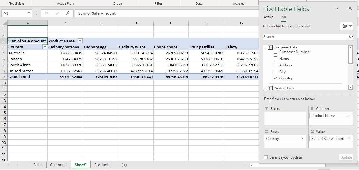
STEP 6: Now setup the following:

• Rows – Country

Click Auto-Detect

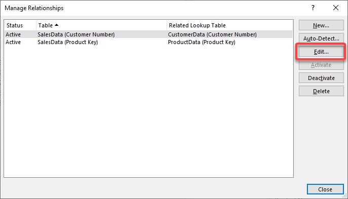
STEP 7: Select Manage Relationships to see what was created automatically

Click Edit

STEP 8: This is cool as the relationship between Sales and Customer tables is correct! Excel is able to link these tables together via the Customer Number columns. Click OK.

Your Pivot Table is all setup thanks to the automatic creation of the relationships between the 3 tables.

 

Automatic Time Grouping

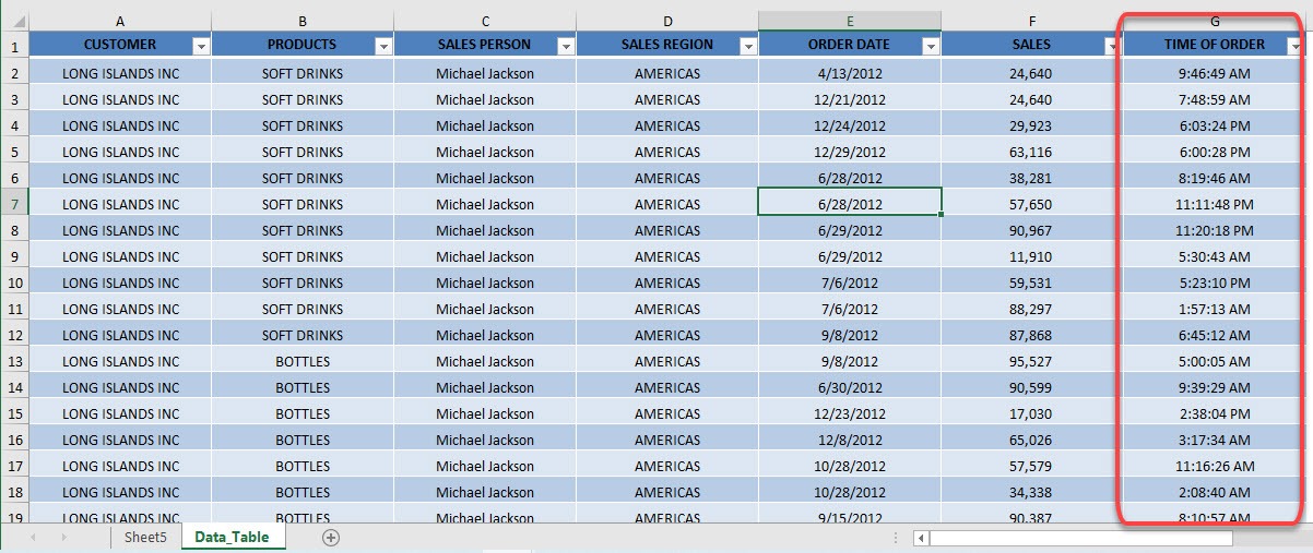
Have a look at our data table. You can see the Time of Order column. Once we create the Pivot Table, Excel is able to group by time periods automatically.

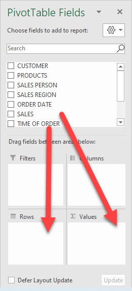
STEP 1: Let us setup the following:

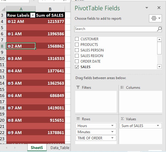
• Rows – Time of Order
• Values – Sales

And just like that, our Sales amounts are grouped by the hour!

 

Search In The Pivot Table Fields List

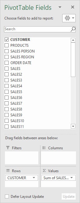
Imagine if we have a lot of PivotTable Fields, there is a new feature that allows us to find it quickly. Making our Pivot Table setup a faster process.

Here is our field list:

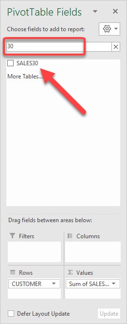
STEP 1: Let us say we want to get the SALES30 field. Just type in 30 in the search box and you have the field right away!

 

Make sure to download our FREE PDF on the 333 Excel keyboard Shortcuts here: