How to Insert the Pi Symbol (π) in Excel

The Pi (π) symbol in Excel is a useful mathematical constant that represents the ratio of a circle’s circumference to its diameter, approximately 3.14159. Excel provides a simple way to work with π in calculations, whether for geometry, trigonometry, or data analysis. In this article, we’ll explore how to insert and use the Pi symbol in Excel formulas efficiently.

Key Takeaways:

• Symbol Dialog Box: Accessible through the Insert tab, the Symbol dialog box lets users search for and insert the Pi symbol with a few clicks.
• Alt Key Shortcuts: For those who prefer keyboard shortcuts, the Alt key combined with a specific numerical code can be employed to insert π swiftly.
• AutoCorrect Function: Excel’s AutoCorrect feature can be configured so that typing a certain text string, like “PIsym”, automatically converts to the Pi symbol.
• Copy-Paste Method: Good old-fashioned copying and pasting from a source that already contains the Pi symbol remains a quick fix.

 

Introduction to the Pi Symbol in Excel

Understanding the Importance of Pi in Excel

Pi, the enigmatic mathematical constant often denoted by the Greek letter π, holds immense significance in Excel. As a reflection of the ratio of a circle’s circumference to its diameter, π is indispensable in a plethora of geometric and trigonometric calculations.

Within Excel, I find it particularly valuable for its precision and versatility, which facilitate a variety of user needs from basic arithmetic to sophisticated scientific computations. Its value, approximately 3.14159, is hard-coded into Excel’s architecture, enabling us to undertake exacting analyses with confidence.

Integrating π into your spreadsheets can transform tedious calculations concerning circular shapes and periodic functions into mere child’s play, making it a fundamental tool in the Excel toolkit.

 

Step-by-Step Instructions to Insert the Pi Symbol

Method 1: Using the Insert Symbol Dialog Box

Using the Insert Symbol Dialog Box is an intuitive method for adding the Pi symbol in Excel. Here’s how I do it:

STEP 1: First, click the cell where the Pi symbol will be placed.

STEP 2: Next, navigate to the Insert tab on the ribbon. Then click on the ‘Symbol’ icon located within the Symbols group to summon the Symbol dialog box.

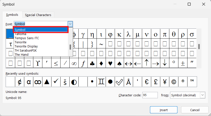
STEP 3: Once the dialog box is open, select “Symbol” from the “Font” dropdown menu for precision.

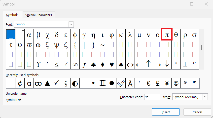
STEP 4: Scrolling through the list, I locate the Pi symbol, which is unmistakable given its distinctive shape.

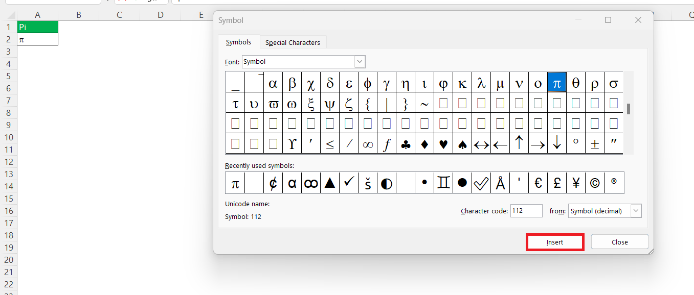
STEP 5: A click on the ‘Insert’ button transfers the Pi symbol into the selected cell in the spreadsheet.

The Symbol dialog box offers a vast array of symbols and I particularly appreciate this method for its directness and the ease of searching for any symbol I need. Plus, it’s one of the best ways to ensure that the symbol is formatted correctly from the start.

Method 2: Typing the Pi Symbol with Alt Key Shortcuts

For those times when speed is of the essence, I often resort to using Alt key shortcuts to insert the Pi symbol in Excel. It’s a lesser-known trick that can save a great deal of time. Here’s the step-by-step process:

STEP 1: Make sure the Num Lock is activated on the keyboard.

STEP 2: Click on the cell where the Pi symbol should go.

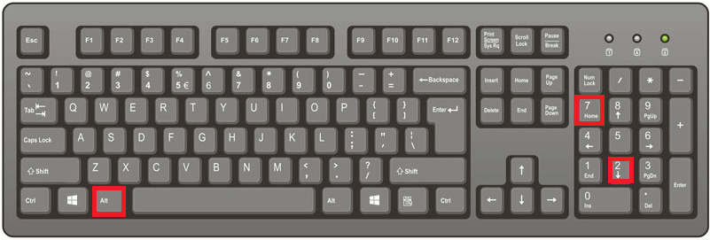
STEP 3: Then, hold down the Alt key. It feels like unlocking a secret door in Excel every time I do this. While keeping the Alt key pressed, I enter 227 on the numeric keypad. It’s fascinating that such a simple sequence can yield the timeless Pi symbol.

STEP 4: Releasing the Alt key brings the symbol π to life in the cell.

It’s important to note that this method requires a numeric keypad, so it may not work on some compact keyboards. The joy of this shortcut is in its simplicity—once memorized, it can become second nature. And it’s not just for Pi; there are other Alt codes for various symbols, making it a universally handy trick.

I’ve found it especially useful when I need to frequently insert the Pi symbol. It’s just a matter of a few keystrokes, and there’s no disruption in my thought process or workflow as I design intricate spreadsheets.

 

Formatting and Customizing the Pi Symbol

Adjusting Pi Symbol Size and Color

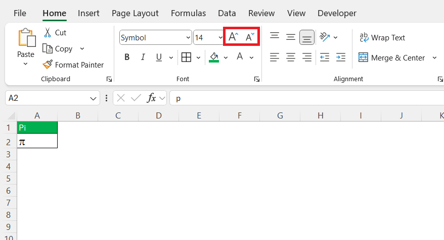
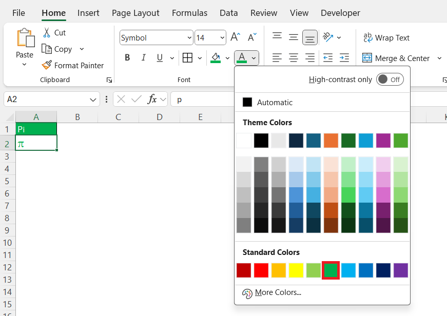
Adjusting the size and color of the Pi symbol can help in drawing focus within spreadsheets or making instructional material more engaging. Here’s how I effortlessly handle these tweaks:

• To change the size, I first select the cell or the Pi symbol itself. Then I head to the ‘Home’ tab and find the font size dropdown in the Font group. A simple selection from the dropdown allows me to make the Pi symbol larger or smaller, in perfect sync with my visual needs.

• Changing color follows a similar easy route. After selecting the symbol, I click on the font color button (usually symbolized by a colored ‘A’ icon) in the Font group on the ‘Home’ tab. I pick the hue that best suits my data presentation, often opting for a color that contrasts well with the rest of the text for better visibility.

When adjusting size and color, I ensure that they contribute to clarity and do not distract from the data. A well-placed highlight or emphasis can turn a mundane spreadsheet into an informative and visually appealing one.

These simple adjustments to the Pi symbol can make a significant impact on how data is perceived and understood. Subtle cues like size and color guide the viewer’s eye toward the most crucial parts of my data or instructions, enhancing the overall communication through the spreadsheet.

 

Alternatives to Insert the Pi Symbol

Employing AutoCorrect Options for Quick Access

For those of us who frequently navigate the world of Greek letters and symbols in Excel, employing the AutoCorrect options can elevate our efficiency. Here’s how I like to set it up:

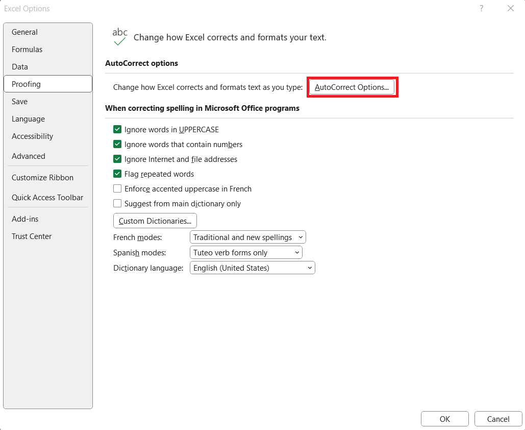
STEP 1: Open the Excel Options dialog by clicking on “File” and then “Options.”

STEP 2: Tapping into the “Proofing” section, I find and click on “AutoCorrect Options…”.

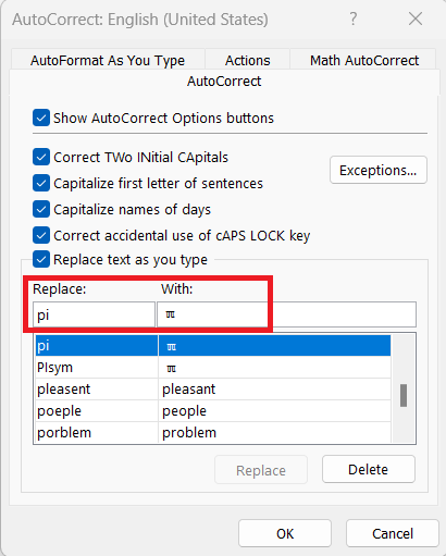
STEP 3: Within the AutoCorrect tab, I type a memorable code, for example, “Pi” in the ‘Replace’ field. This will be my shortcut text.Next, I enter the Pi symbol into the ‘With’ field.

And now, each time I type “Pi” , it magically transforms into π. The AutoCorrect function becomes my silent, incredibly efficient assistant, one that never fails to save me time and guard against the monotony of manual insertions.

This feature proves itself to be a game-changer, especially when working on detailed spreadsheets that require frequent insertion of special symbols. It’s a perfect example of how a deep understanding of one’s tools can streamline complex tasks and bring forth productivity gains in unexpected places.

 

Handy Tips for Working with Pi in Formulas and Functions

Incorporating Pi into Common Excel Functions

In my work with Excel, incorporating Pi into common functions is like adding a secret ingredient that amplifies the capabilities of my spreadsheets. Here are some examples:

• Calculating Circumference and Area of Circles: To calculate a circle’s circumference or area, I just wrap the PI function with multiplication. For instance, =PI()*D4 gives me the circumference when ‘D4’ is the diameter, and =PI()*POWER(radius, 2) hands me the area on a silver platter when ‘radius’ is the radius of my circle.
• Trigonometric Operations: Trigonometry and Pi go hand in hand. When I’m dealing with sine, cosine, or tangent functions, embedding Pi can refine the outcome. If I need the sine of Pi, I simply type =SIN(PI()).
• Scientific Calculations: For more complex scientific computations like waveforms or cycles where Pi is a core component, I directly integrate it using the PI function within a formula. This ensures that the calculations are as precise as they need to be.
• Financial Models: Sometimes it’s about angles and curves in financial models. Here, I also turn to the trusty PI function for geometric growth rates or periodic payments.
• Stochastic Processes: For models involving randomness like the Monte Carlo simulation, Pi can sometimes sneak into the calculation of probabilities or modeling of circular patterns.

Understanding how Pi interacts with other Excel functions allows me to harness its full potential. It’s not just about plugging in a number; it’s about recognizing Pi’s omnipresence in anything revolving around cycles, circular shapes, and periodicity.

Remember, Excel’s precision with Pi impresses even across different scientific fields, allowing us as users to engage in calculations that are not just accurate but also meaningful.

Preventing Errors When Utilizing Pi in Calculations

While utilizing Pi in Excel calculations, I’ve found that precision and attention to function structure are pivotal to avoiding errors. Here’s what I focus on to prevent missteps:

• Consistency in Units: Ensuring that all units within my formulas are consistent is paramount. For instance, if I’m calculating area or circumference, I make sure that I have not mixed up radii, diameters, or circumferences in different units.
• Use of Brackets: I always use brackets properly to define the order of operations in my formulas. It disambiguates the computation sequence, especially when the PI function is combined with other functions or constants.
• Avoiding Rounding Errors: Since Pi is a transcendental number, rounding it can lead to inaccuracies. I use the PI function directly rather than entering a rounded approximation. For display purposes, however, rounding the final result with the ROUND function is acceptable and sometimes necessary.
• Verifying Formulas: A step-by-step verification of my formulas is something I never skip. Excel’s Formula Auditing tools come in handy for tracing precedents and dependents, helping me ensure everything is linked appropriately.
• Use of Named Ranges or Constants: If I’m using Pi multiple times across my workbook, I define a named range or constant to avoid repeated formula entry. This minimizes the risk of accidental misentry and keeps all references uniform.

By upholding these simple yet effective practices, I help ensure that my calculations with Pi are as robust and error-free as can be. After all, accuracy in the digital representation of Pi resonates through to the accuracy of the overall outcomes.

Every calculation in Excel, especially those involving constants like Pi, needs meticulous verification because even the tiniest error can cascade through a spreadsheet with unforeseen consequences. It’s the precision in these details that maintains integrity in my computational endeavors.

 

FAQs

How do you write pi in Excel?

To write pi in Excel, simply enter the PI function into a cell by typing =PI() and press Enter. This inserts pi to the full precision of Excel’s capabilities, which is typically 15 decimal places.

How do you insert the symbol pi?

To insert the Pi symbol in Excel, go to the Insert tab, click on the Symbol button, and from the Symbols dialog box, select Greek and Coptic from the Subset dropdown. Find and click the Pi symbol (π), then click Insert.

Can Excel Calculate PI?

Yes, Excel can calculate Pi using the built-in PI function. Just type =PI() into a cell and hit Enter; Excel will return the value of Pi.

How to Do type sin(π) in Excel?

To calculate the sine of Pi in Excel, type the formula =SIN(PI()) into a cell and press Enter. Excel will compute the value, which should display as 0, since the sine of Pi is mathematically zero.

What is the Unicode for PI in Excel?

The Unicode for Pi in Excel is 03C0. To insert the Pi symbol using this code, type =UNICHAR(960) or =UNICHAR(hex2dec("03C0")) into a cell and press Enter.