Excel Pivot Cache Explained

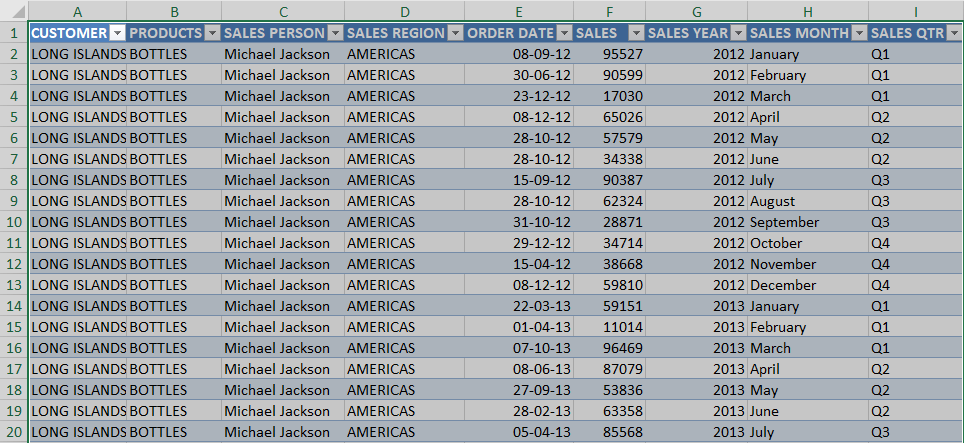
Whenever you make a change to your dataset (updating data, adding more rows or columns), you have to manually refresh your Pivot Table to have your changes reflected. Why is that? I’m going to explain to you the concept of the Pivot Cache. Join me in understanding this concept with some quick illustrative examples below!

• Pivot Tables Store a Snapshot of Your Data – When you create a Pivot Table, Excel automatically creates a Pivot Cache, which stores a snapshot of the data source.

• Improves Performance and Speed – The Pivot Cache allows Pivot Tables to work quickly and independently of the original data source, especially useful for large datasets.

• Multiple Pivot Tables Can Share One Cache – If built from the same source range, Pivot Tables can share a cache, reducing file size and improving consistency.

• Cache May Not Update Automatically – If you change the source data, you’ll need to refresh the Pivot Table to update the cache and reflect changes.

• Pivot Cache Increases File Size – Since it duplicates source data, having many Pivot Tables with different caches can bloat your workbook unless managed properly.

What is Pivot Cache?

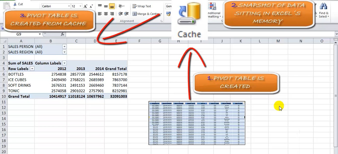
STEP 1: Why is there a need to refresh the Pivot Table? Let us look at this sequence of events below:

• You invoke the creation of the Pivot Table
• Then a snapshot of that data in that point in time is stored in the Cache
• The Cache content is the basis of how the Pivot Table is created

You do not see the Pivot Cache as this runs in the background.

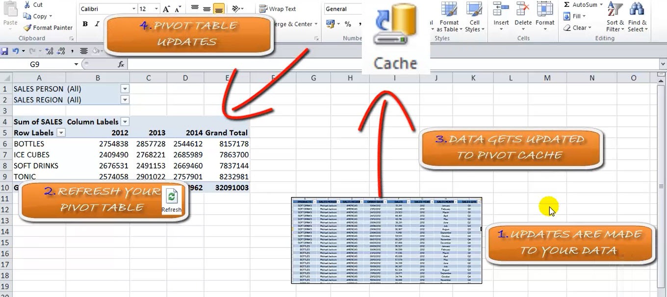
STEP 2: Now what happens when you update the source data?

• Your source data is updated
• You invoke the refreshing of the Pivot Table
• Then a snapshot of that data in that point in time is stored in the Cache
• The Pivot Table is updated based on the Cache

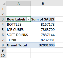
When you create Pivot Table in Excel, a Pivot Cache is created automatically. It is a replica of the original source data but it is not visible to us. When you make changes to the Pivot Table, it uses Pivot Cache and not the original source data.

Even though this makes Excel very responsive and quick to change, it increases the file size to almost double.

 

Sharing a Pivot Cache

When you create multiple Pivot Tables using the same source data in a workbook, Excel creates a single Pivot Cache and re-uses it for all Pivot Tables.

The advantage of sharing a Pivot cache is that it prevents duplication but it creates several disadvantages as well:

• When you refresh one Pivot Table, all other Pivot Tables get refreshed.
• When you group one field in Pivot Table, it gets grouped in other Pivot Tables.
• When you insert a calculated field in Pivot Table, it appears on all other Pivot Tables.

If these disadvantages create a hindrance for you, you can simply create multiple Pivot caches for multiple Pivot Tables. To do so, follow the steps below:

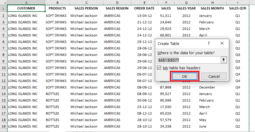
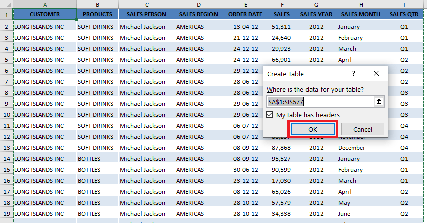
STEP 1: Click anywhere on the data source and press Ctrl + T to create a table. Click OK.

STEP 2: Go to the Table Design tab, you will see the Table Name box displaying the name (Table1) assigned to the table.

STEP 3: Select Summarize with PivotTable.

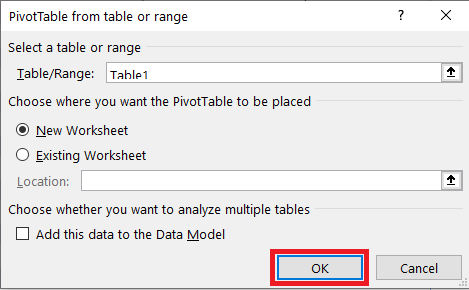
STEP 4: In the PivotTable dialog box, click OK.

Pivot Table and its cache will be created. Before you create another PivotTable, you need to covert the table back to range.

STEP 5: Go to Table Design Tab > Convert to Range.

STEP 6: Again convert the range back to a table.

Excel will assign a different name to the table – Table2.

Now you can create another Pivot Table using the data from Table2.

Since the tables have different names, Excel will create separate caches for them!

 

Count the Pivot Cache in Workbook

How to do how many pivot caches are present in your workbook? Excel can count them for you using a simple VBA code.

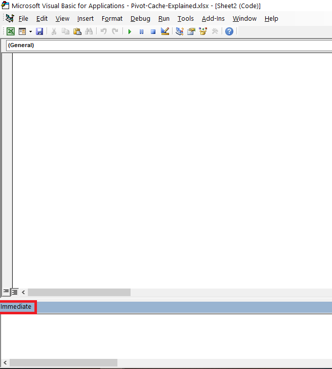
STEP 1: Press Alt + F11 to open the Visual Basic window.

STEP 2: Press Ctrl + G to open the Immediate window.

STEP 3: Enter the following code:

?ActiveWorkbook.PivotCaches.Count

STEP 4: Press Enter.

The result will be displayed below the code!

 

Reduce Excel File Size

The only issue that you face while using Pivot cache is that it doubles the size of the Excel file. This problem can easily be solved by deleting the original source data. This will reduce the file size significantly!

The Pivot Table will remain intact and you can easily use it.

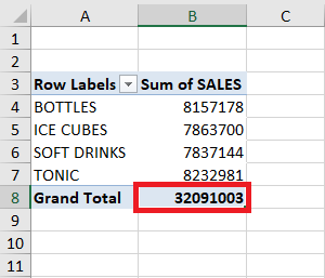
If you want to get the source data back, double click on the grand total value in the unfiltered Pivot Table.

This will paste the original source data into a new worksheet for you.

Frequently Asked Questions

What is a Pivot Cache in Excel?
A Pivot Cache is a memory-resident copy of the data source used by Pivot Tables. It enables efficient filtering, summarizing, and slicing of data.

Can multiple Pivot Tables use the same Pivot Cache?
Yes, if they are based on the same data range or table, Excel will reuse the same Pivot Cache to optimize performance.

How do I refresh a Pivot Cache?
Right-click the Pivot Table and choose “Refresh” to update the cache with any changes from the source data.

Why is my Excel file getting so large with Pivot Tables?
Each Pivot Cache stores a copy of the source data. If you have multiple Pivot Tables with separate caches, your file size can increase significantly.

Can I control or view Pivot Caches in Excel?
Excel doesn’t provide a direct interface, but you can manage Pivot Caches using VBA macros to check how many caches exist or to consolidate them.