Pivot Table Filter: Top 5 Customers

You can easily filter your Pivot Table to show your Excel Pivot Top 5 customers or Top X Customers. There are lots of different Value Filters to choose from: Filter Items by Value, Filter Items that make up a Specific Percentage of Value, Filter Items that make up a Specific Value.

Key Takeaways:

• Highlight Key Performers: Using a “Top 5” filter in a Pivot Table helps you quickly identify your highest-performing customers based on metrics like sales or revenue.
• Dynamic Filtering: Pivot Table filters allow you to dynamically update the top 5 customers as data changes, ensuring the results always reflect the most current information.
• Customizable Criteria: The “Top 5” filter can be adjusted to focus on other rankings or percentages, such as the top 10 customers or the top 20% of sales contributors, providing flexibility for analysis.

Filter Items by Value

You can easily create Pivot Table in Excel to summarize your data and use the filter option to get the Top/Bottom X values from the data.

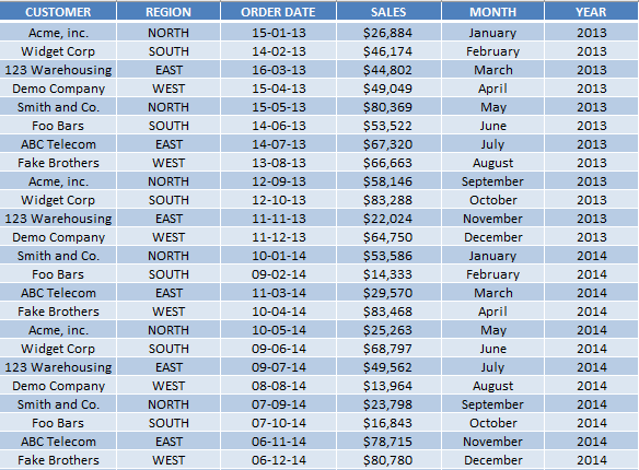
Here is an example of sales data of a company:

You can use the in-built filter to display the pivot table top 5 by sales value.

Let’s see how you can create a pivot table and display Excel top 5 values and names!

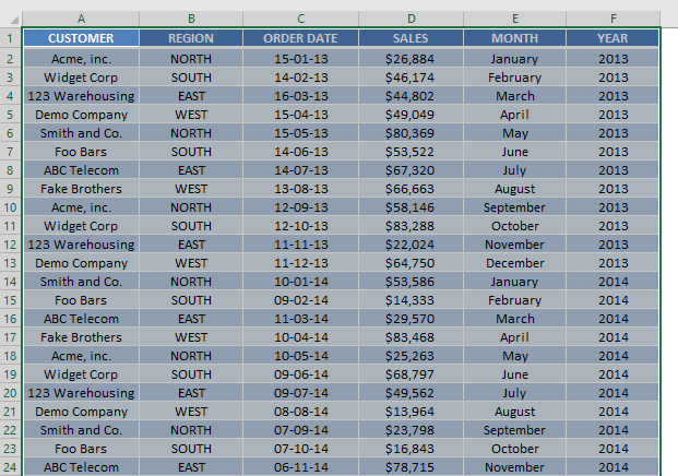
STEP 1: Select all Cells in the Data Table.

STEP 2: Go to Insert > Pivot Table.

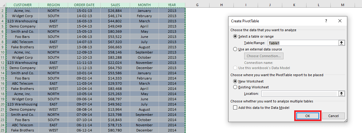
STEP 3: In the Create PivotTable dialog box, Click OK.

You don’t have to change any default setting.

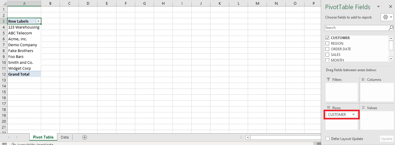
STEP 4: In the PivotTable Fields dialog box, drag and down Customer Label in Row Area.

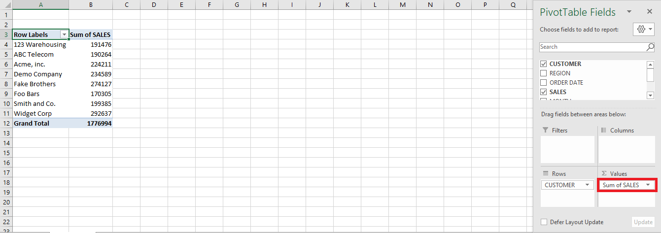
STEP 5: Now, drag and down Sales Label in Column Area.

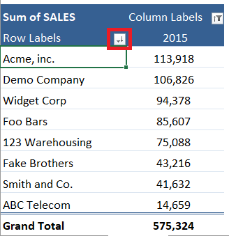
Now, you have an entire list of total sales by different customers. To find the Excel Pivot Top 5 customer by sales, follow the steps below:

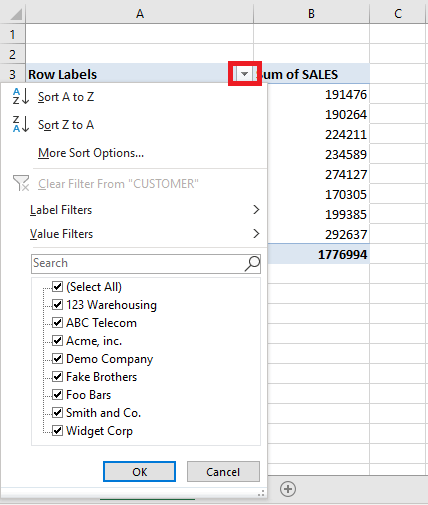
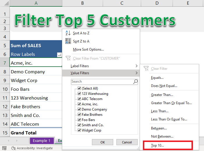
STEP 6: Click on the filter button next to Row Labels.

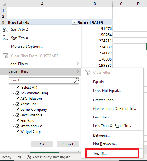
STEP 7: Go to Value Filters > Top 10.

STEP 8: In the Top 10 Filter (CUSTOMER) dialog box, type 5 and Click OK.

 

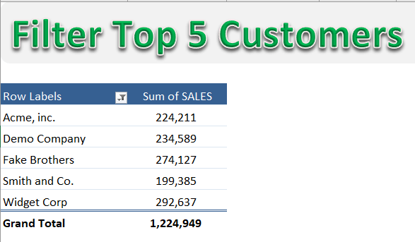
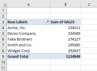
Your pivot table is now filtered!

 

Now, that you have a list of Excel Pivot Top 5 customers by sales. Let’s move forward and understand what else can be done using this Top 10 filter in Excel.

The Top 10 filter is super flexible and you can easily filter the data to get Bottom 2, Top 80%, etc.

 

Bottom 2 Customer

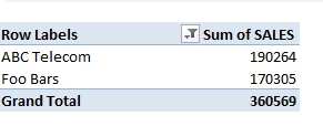
In the Top 10 Filter dialog box, select Bottom from the dropdown and type 2.

The result will be as shown below:

 

Filter Items that make up a Specific Percentage of Value

Instead of displaying Top or Bottom X values, you can also show a specific portion of the grand total amount.

To display the top-selling customers contributing to 2% of the total sales amount:

STEP 1: Click on the Filter buttons in the Pivot Table.

STEP 2: Go to Value Filter > Top 10.

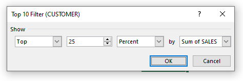
STEP 3: In the Top 10 Filter dialog box:

• In the first field, select Top.
• In the second field, type 25.
• In the third field, select Percent.
• In the fourth field, select Sum of SALES.

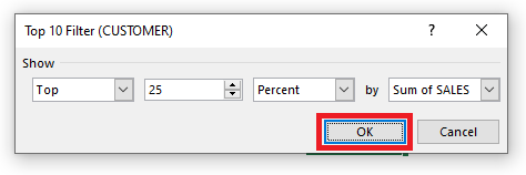
STEP 4: Click OK.

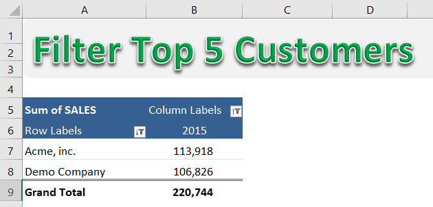
This will provide you with a list of top customers that represent 25% of the sales.

Filter Items that make up a Specific Value

You can use this filter to get a list of top customers that accounts for a specific value say $300,000.

To display the top customers that account for $300,000:

STEP 1: Click on the Filter buttons in the Pivot Table.

STEP 2: Go to Value Filter > Top 10.

STEP 3: In the Top 10 Filter dialog box:

• In the first field, select Top.
• In the second field, type 300000.
• In the third field, select Sum.
• In the fourth field, select Sum of SALES.

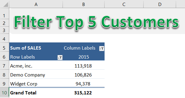
Here, is the result!

 

Frequently Asked Questions

How do I filter a Pivot Table to show only the top 5 customers?

To filter a Pivot Table by the top 5 customers, click the dropdown arrow on the field you want to filter (e.g., “Customer Name”). Select Value Filters > Top 10, then set the filter to “Top 5” and choose the metric to rank by, such as “Sum of Sales.” Click OK, and the table will update to show the top 5 customers based on the selected metric.

Can I change the “Top 5” filter to show a different number of customers?

Yes, you can adjust the number of customers displayed by reopening the filter settings. Go to Value Filters > Top 10, and change the number from 5 to any desired value (e.g., 10 or 3). This flexibility allows you to customize your analysis based on your specific needs.

Does the “Top 5” filter update automatically when data changes?

Yes, the filter dynamically updates when you refresh the Pivot Table. If new data is added or existing data changes, the top 5 customers will be recalculated based on the updated metrics, ensuring that the table always reflects the most current information.