Prepare Data for Excel Pivot Tables

• Tabular Format – your data is organized as a list with labeled columns
• No Gaps – no blank columns and no blank rows
• Tables – use this for structured referencing, Excel automatically updates as more rows and columns are added

Then you will be able to harness the full power of Pivot Tables!

Exercise Workbook:

---

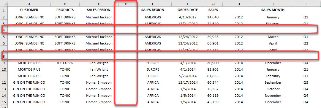
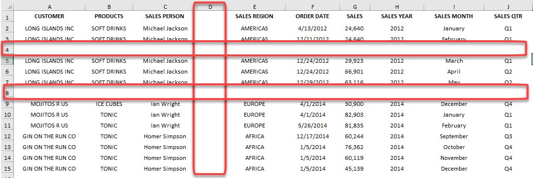
Let us go over the principles one by one! Here is our data set:

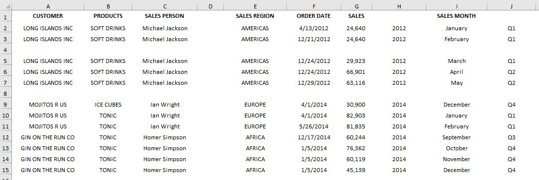
You can see that it has a couple of issues. There are 2 columns without label headers:

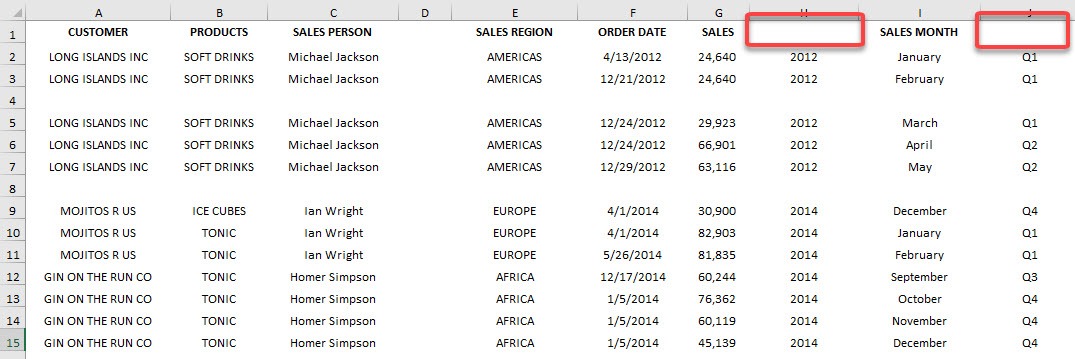
Then we also have 1 blank column and 2 blank rows. Let us get this data cleaned up!

STEP 1: Let me quickly demonstrate to you first that we cannot use this set of data to create a Pivot Table.

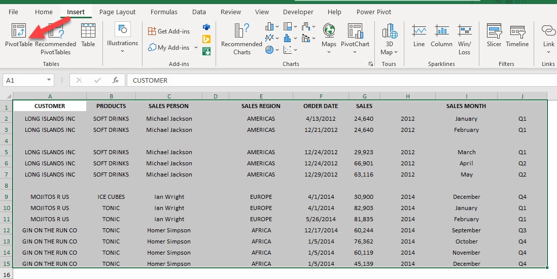
Select the entire table of data and Go to Insert > Tables > PivotTable

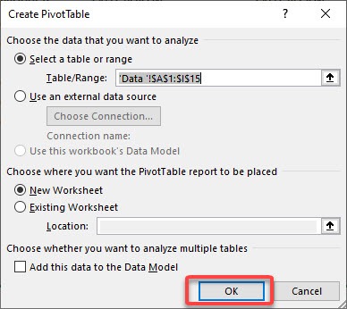
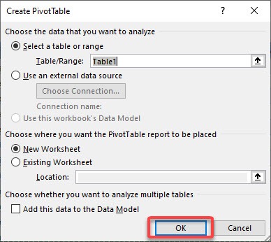
STEP 2: Click OK

We get this error message because our data is not Pivot Table ready. Let us fix that!

 

Tabular Format

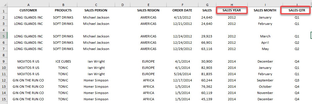
STEP 3: Let us follow the Tabular Format principle. For the blank column headers, add SALES YEAR and SALES QTR:

 

No Gaps

STEP 4: Now for the No Gaps principle, delete the blank column D and delete the blank rows 4 and 8.

Our data is now looking good!

 

Tables

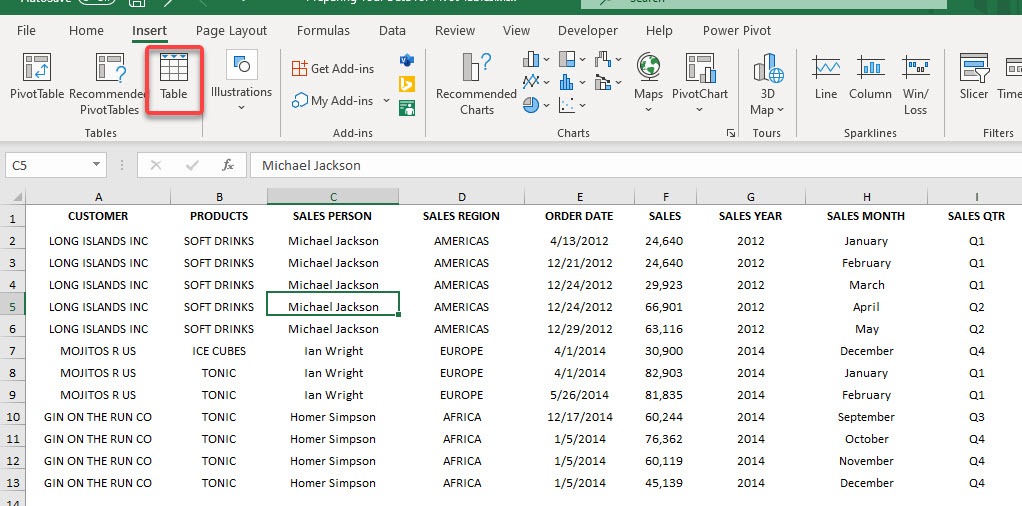
STEP 5: Go to Insert > Tables > Table to convert this into an Excel Table

STEP 6: Click OK

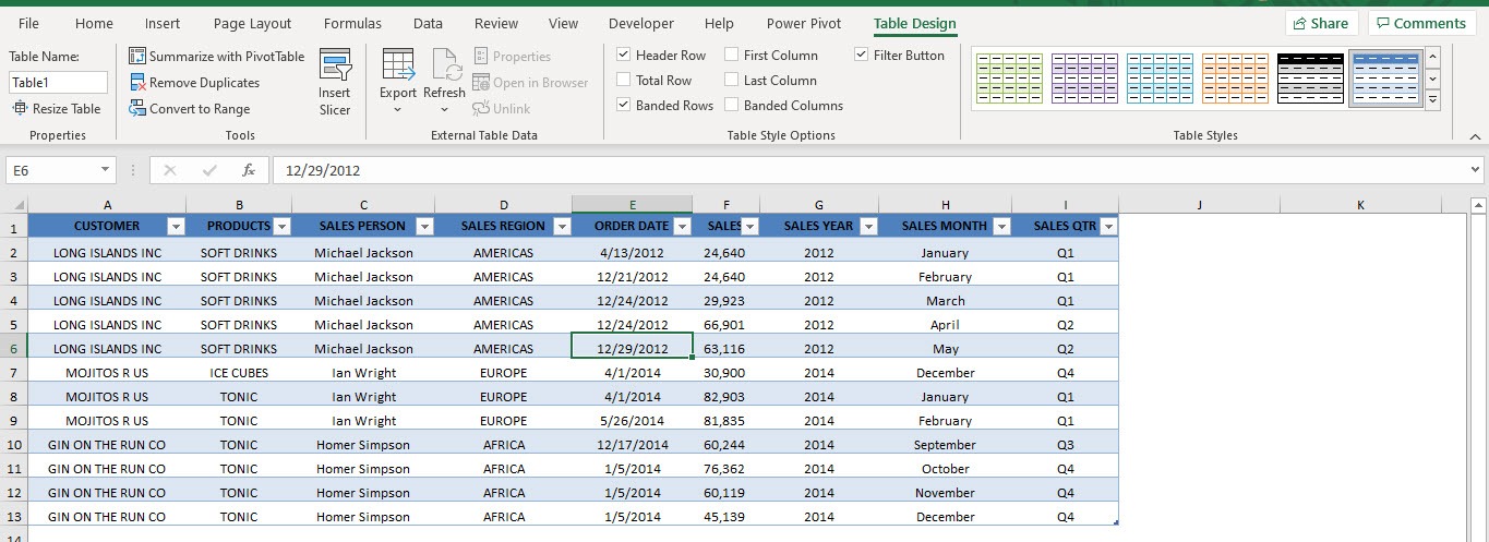
We have our Excel Table ready! You get a lot more feature here like sorting, filtering, Table Styles to name a few.

Now that you have prepared for data, let’s try and create a Pivot Table again!

 

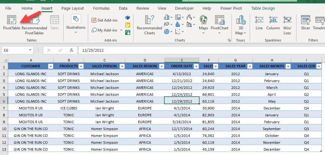
STEP 7: Go to Insert > Tables > PivotTable

STEP 8: Click OK to insert the Pivot Table into a new worksheet.

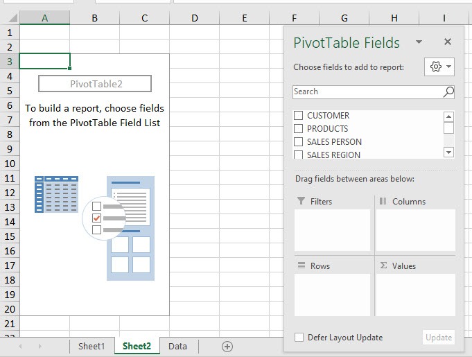
And we are all set!