Product in Excel Pivot Tables

Our main methodology will be using the Product in Pivot Table. What this does is it will multiply all the values together.

Exercise Workbook:

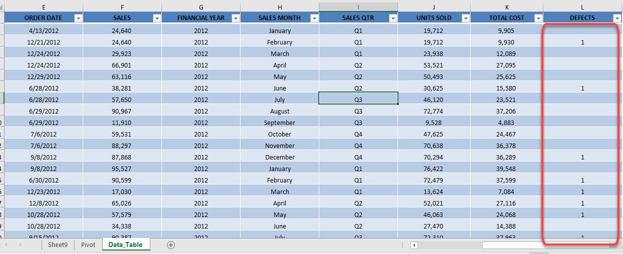
Here is our data set. Notice that I have added a Defects column. If there is a defect that day, we simply mark it as 1. This will be crucial once we use the Product function later.

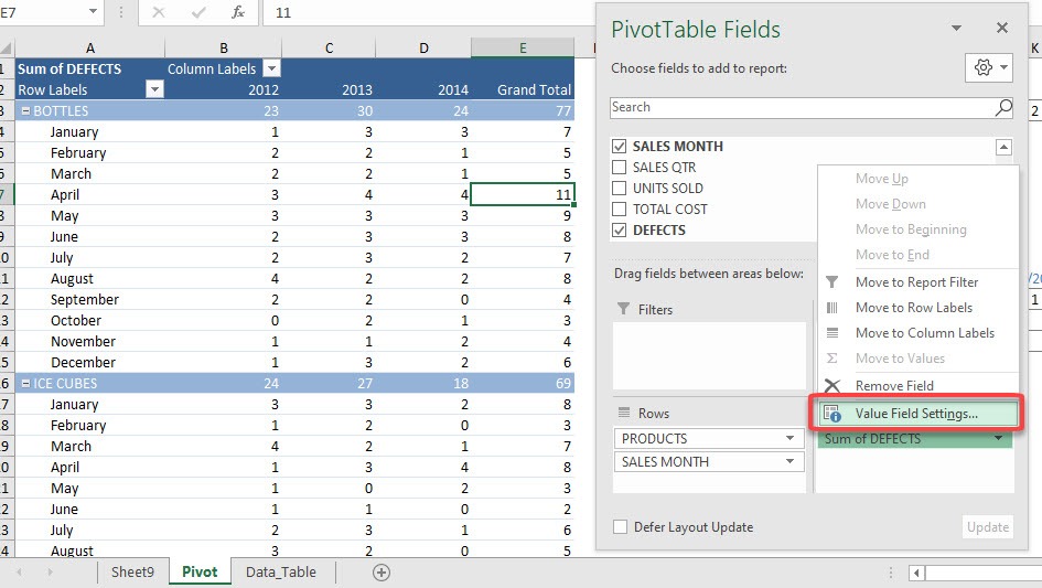
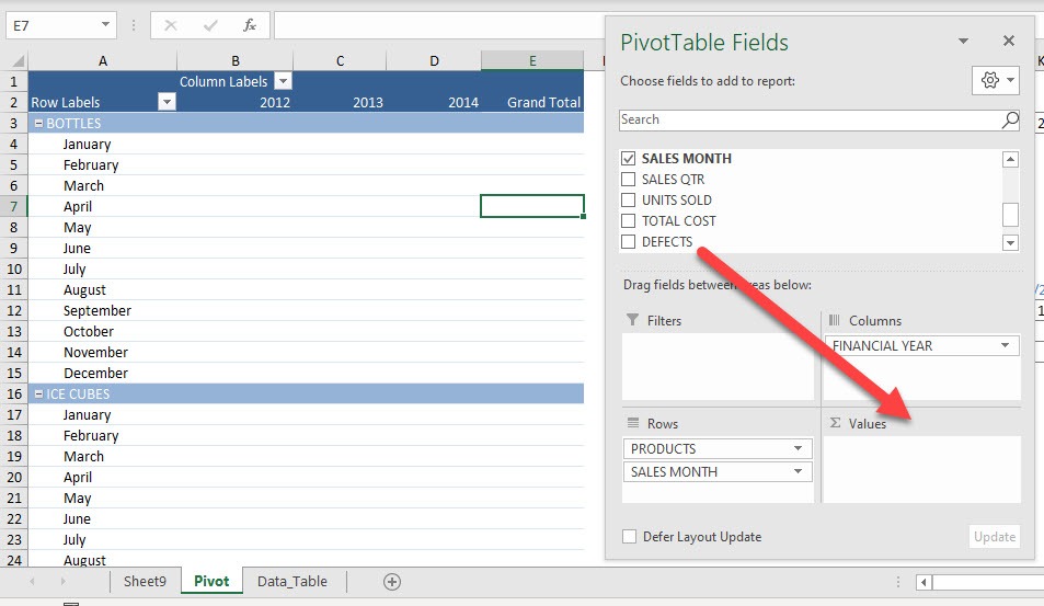
STEP 1: This is our Pivot Table setup. Drag Defects to the Values area:

STEP 2: It will default as Sum of DEFECTS. Click on the arrow and select Value Field Settings

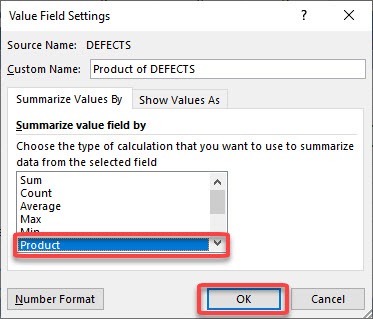
Select Product and click OK.

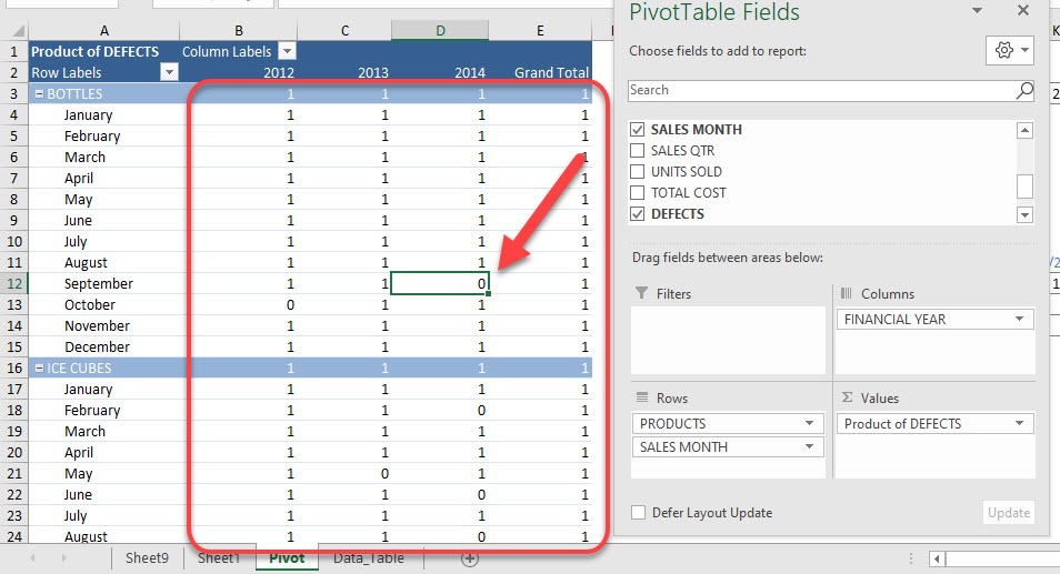
STEP 3: Now what Excel has done is for that specific duration, it has multiplied all the Defect values. So if any row for that specific duration has a 1, then the result in this Pivot Table is a 1 as well.

We love the ones that show zero because that means there are no defects! For example, would be for Bottles during the month of September 2014. Double click on it to see more details!

You can see that in the data breakdown for September 2014, there are no defects! This is why the Product result is 0.

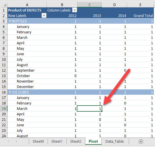
Now try double-clicking on Ice Cubes during the month of March 2013:

You can see it has defects, so which is why the Product result when you multiply them together is 1.

Make sure to download our FREE PDF on the 333 Excel keyboard Shortcuts here:

Bryan

Bryan Hong is an IT Software Developer for more than 10 years and has the following certifications: Microsoft Certified Professional Developer (MCPD): Web Developer, Microsoft Certified Technology Specialist (MCTS): Windows Applications, Microsoft Certified Systems Engineer (MCSE) and Microsoft Certified Systems Administrator (MCSA).

He is also an Amazon #1 bestselling author of 4 Microsoft Excel books and a teacher of Microsoft Excel & Office at the MyExecelOnline Academy Online Course.