Whenever I wanted to print my Excel worksheet for a report, I usually had to trim down the data and do changes like hiding the columns so it could fit into one page.
Other common scenarios would be, hiding employee salaries or filtering out specific customer data.
It is cumbersome because after printing it out I had to undo the layout changes one by one!
Thankfully Excel has Custom Views that lets you revert and save your layout changes in a single click!
STEP 1: You need to set a default view first.
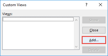
Once you have the layout that you use most of the time, go to View > Custom Views:
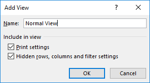
STEP 2: Click Add to create a new Custom View.
Type in Normal View and click OK.
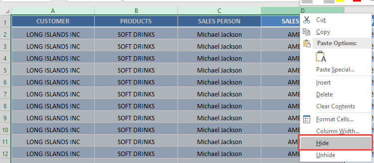
STEP 3: In preparation for the second Custom View, select the first 4 columns, right click and select Hide.
STEP 4: Go to View> Custom Views:
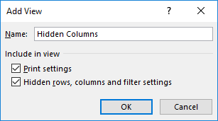
STEP 5: Click Add to create a new Custom View.
Type in Hidden Columns and click OK.
STEP 6: Let us now try out our Custom Views in action.
Go to View > Custom Views.
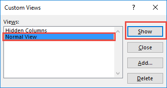
Select Normal View and click Show.
You can see all of the columns displayed.
STEP 7: Now let us try the second custom view.
Go to View > Custom Views.
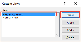
Select Hidden Columns and click Show.
The columns are hidden right away in a click! Imagine if you have multiple layout customizations, it is now doable and saved in a Custom View!

Bryan
Bryan Hong is an IT Software Developer for more than 10 years and has the following certifications: Microsoft Certified Professional Developer (MCPD): Web Developer, Microsoft Certified Technology Specialist (MCTS): Windows Applications, Microsoft Certified Systems Engineer (MCSE) and Microsoft Certified Systems Administrator (MCSA).
He is also an Amazon #1 bestselling author of 4 Microsoft Excel books and a teacher of Microsoft Excel & Office at the MyExecelOnline Academy Online Course.


