How to Create Reference Tables in Excel – Step by Step Guide

In my journey with Excel, I’ve often found myself dealing with large datasets that require a level of organization and efficiency that can be challenging. One of the most powerful tools I’ve discovered to manage this complexity is the reference table. This tool has revolutionized the way I handle data, enabling me to cross-reference and look up information with ease. Let me take you through how I’ve mastered using reference tables in Excel and how they can help you too.

Key Takeaways:

• Reference tables in Excel simplify managing complex datasets by enabling easy cross-referencing and lookups.
• Structured references enhance formula readability and efficiency by using table names and column headers instead of cell coordinates.
• INDEX and MATCH functions offer more versatility than VLOOKUP, especially for non-vertical data lookups.
• Dynamic named ranges adjust automatically as data is added or removed, keeping your reference tables up-to-date.
• Adopting best practices, such as naming tables and testing lookups, ensures your reference tables remain effective and error-free.

 

Unveiling the Magic of Structured References in Excel

What is a Structured Reference?

Structured references are akin to a secret spellbook enhancing the wizardry of Excel tables. They allow you to interact with table data by using table names and column headers, rather than traditional cell coordinates (like A1, B2).

To understand where the magic lies, consider an Excel Table as a dynamic entity; when structured references are employed, they automatically adapt to changes such as added or removed data, reducing the risk of errors and manual adjustments.

Imagine labeling a potion bottle with “Dragon’s Breath” instead of “Bottle #3” – that’s structured referencing for you; it speaks the language of your data.

Why Use Structured References?

Using structured references is like having an assistant who keeps your formulas meaningful and manageable. They elevate efficiency because they are self-adjusting – if I add rows or columns to a table, the references update without any extra work on my part

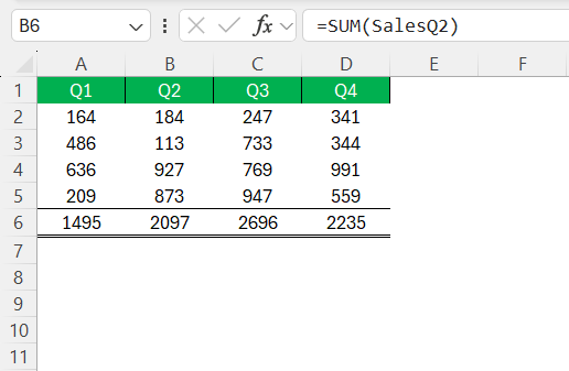
Imagine recalculating your budget when adding expenses; structured references do the heavy lifting, updating sums and averages automatically. They also increase formula readability; it’s easier to decipher a formula that reads “Sales[Q2]” versus “B2:B5”, making your Excel experience less about interpreting cryptic cell addresses and more about understanding the story your data tells.

Reports become clearer, data analysis gets streamlined, and the door opens to a level of dynamism that classic referencing can’t touch.

 

Setting Up A Reference Table

My First Reference Table

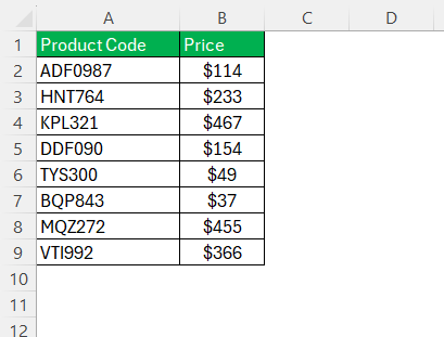
I remember the first time I set up a reference table—it was a game-changer. I had a list of products with corresponding prices, and I needed to create an invoice that would automatically fill in the product prices based on the product codes entered. The idea of manually entering prices each time felt daunting, so I turned to a reference table.

Here’s what I did:

STEP 1: Create the Reference Table: I created a simple table with two columns: one for the product codes and one for the prices. This table was the backbone of my data lookup.

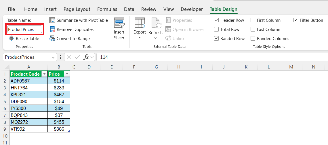
STEP 2: Naming the Table: To make it easier to reference, I named the table (e.g., ProductPrices). This step is crucial because it allows for more straightforward formulas later on.

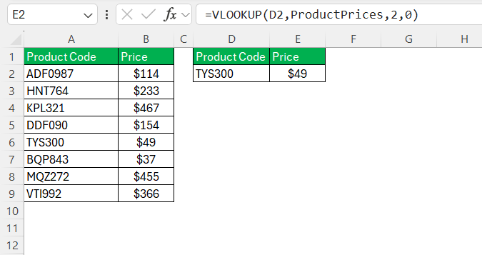
STEP 3: Using VLOOKUP: I used the VLOOKUP function to pull the price from the reference table whenever I entered a product code in my invoice. It was as simple as:

=VLOOKUP(D2, ProductPrices, 2, FALSE)

This formula looks for the product code in cell D2, checks the ProductPrices table, and returns the price from the second column. The FALSE ensures that the lookup is exact.

Enhancing Efficiency with INDEX and MATCH

As I became more comfortable with reference tables, I started exploring other functions like INDEX and MATCH. These functions provide more flexibility and power, especially when dealing with complex datasets.

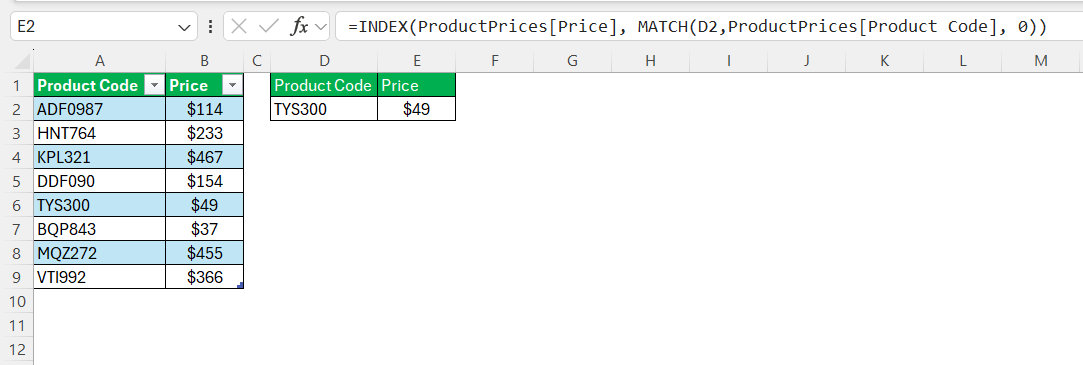
Unlike VLOOKUP, which only searches vertically, the INDEX and MATCH combo allows for more versatility. MATCH finds the position of a value in a row or column, and INDEX returns the value at that position in a specified range. This combination was particularly useful when I needed to look up values in tables where the lookup column wasn’t the first column.

Here’s a quick example:

=INDEX(ProductPrices[Price], MATCH(D2, ProductPrices[ProductCode], 0))

This formula first finds the product code in the ProductPrices table using MATCH, then uses INDEX to return the corresponding price.

 

The Power of Structured References

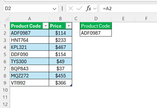
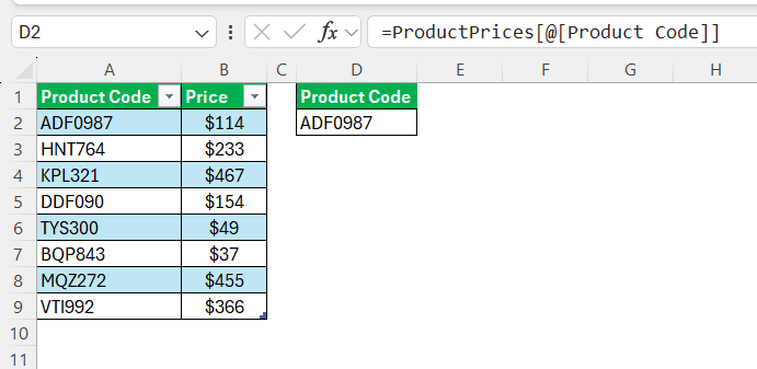
One of the features I’ve grown to appreciate is Excel’s structured references, which allow you to refer to table columns by their headers rather than cell addresses. This makes your formulas easier to read and less error-prone. For example, instead of using:

=A2

I can write:

=ProductPrices[@[Product Code]]

This small change made my formulas more intuitive, especially when sharing my workbook with colleagues.

Dynamic Reference Tables with Named Ranges

As I dealt with more dynamic datasets, I realized that sometimes my reference table would grow as new data was added. I started using named ranges that automatically adjust as data is added or removed

Excel’s Table feature automatically creates dynamic named ranges, but when I needed even more control, I used formulas like OFFSET and INDEX to define dynamic ranges.

 

My Go-To Reference Table Best Practices

Over time, I’ve developed a few best practices to ensure that my reference tables are effective and easy to maintain:

1. Keep it Simple: Start with a clear structure. Each table should have a specific purpose, with clearly defined columns.
2. Name Your Tables: Always name your tables. It makes your formulas cleaner and easier to understand.
3. Use Structured References: Whenever possible, use structured references to make your formulas more readable.
4. Test Your Lookups: Before relying on your reference tables, always test your lookups with a few sample data points to ensure they’re working correctly.
5. Document Your Work: Especially in larger workbooks, document what each reference table is used for. This will save time when you or someone else needs to modify or update the workbook later.

 

Battling Error Dragons: Tips and Tricks

Debugging Common Structured Reference Pitfalls

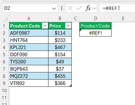
Every Excel sorcerer occasionally encounters a misfired spell or two. When dealing with structured references, a few common pitfalls await. They often arise from the dynamic nature of tables adjusting to data changes, or syntax errors that go unnoticed until the dreaded ‘#REF!’ materializes.

To debug these, I scrutinize the formula and cross-reference it with the table’s anatomy. I ensure the table name is accurate and the columns still bear the names assumed by the formula. It’s akin to checking potion ingredients—if one is incorrect or missing, the entire concoction could turn to sludge.

It’s also prudent to verify the ‘@’ character’s usage, particularly in more complex formulas traversing rows. Remember, ‘@’ is the key to the current row’s context, and misplacing it can alter the intended incantation for the data set dramatically.

Lastly, I inspect the table for rogue rows or columns that might have slipped in or out of the structural range. With structured references being automatically elastic, unintended data additions or deletions can play havoc with the intended calculations.

 

FAQ: Your Treasure Map to Excel Mastery

How to reference a table in Excel?

To reference a table in Excel, click any cell within your data and press Ctrl+T to create the table. Name it in the ‘Table Name’ box under the ‘Table Tools > Design’ tab. Then use the table name and column headers in formulas—for instance, “TableName[HeaderName]” directly references a specific column.

How Do I Create a Structured Reference?

To create a structured reference, convert your range into a table by clicking any cell in the data and pressing Ctrl+T. Define the table with a name, then in formulas, refer to table elements using the name and column headers like “TableName[ColumnName]”. Excel then displays the structured reference.

Can I Use VLOOKUP with Structured References?

Yes, you can use VLOOKUP with structured references in Excel. Instead of cell ranges, use the table name and column headers for lookups—for example, “VLOOKUP(lookup_value, TableName[[#All],[LookupColumn]:[ResultColumn]], column_number, FALSE)” where ‘TableName’ is your table’s name.

What’s the Difference Between Relative and Absolute References in Tables?

Relative references in tables adjust based on the position where they’re used, ideal for copying formulas across multiple cells. Absolute references, tweaked by repeating the column identifier, lock onto a specific part of a table regardless of the formula’s location, ensuring consistency.

How Can I Avoid #value! Errors in Table Formulas?

To avoid #VALUE! errors in table formulas, ensure that the data types in your columns match the formula’s expectations. For structured references, verify proper syntax and that any specific row references use the ‘@’ symbol appropriately. Double-check that all table names and column headers are correct and exist.