Remove Second Hyphen with Excel’s SUBSTITUTE Formula

There are times where I needed to remove the nth occurrence from my text.  For example, I would like to how to remove dashes in Excel – it’s 2nd occurrence.

Normally I would have to find the second hyphen, split the text based on the hyphen’s location, merge the remaining parts together….pfff….it’s just a headache and prone to errors!!

The SUBSTITUTE formula in Excel can actually do this for you! You might be thinking, “How can substitute remove dash in Excel?”

The secret is, we use SUBSTITUTE to replace our target character with an empty string!

 

Let’s get familiar with the syntax of the Substitute Function in Excel!

What does it do?

Substitutes new_text for old_text in a text string.

Formula breakdown:

=SUBSTITUTE(text, old_text, new_text, [instance num])

What it means:

• text – the cell that contains the character you want to substitute
• old_text – the character you want to change
• new_text – the new character you want to place
• [instance num] – the occurrence of the old text you want to replace

---

 

I explain how you can do this and please go to the bottom of the page to see the animated gif tutorial:

Watch it on YouTube and give it a thumbs-up!

STEP 1: We need to enter the Substitute function next to the cell that we want to clean the data from:

=SUBSTITUTE

 

STEP 2: Enter the first argument of the SUBSTITUTE function: text

Which text do we want to change?

Reference the cell that contains the text or value:

=SUBSTITUTE(C9,

STEP 3: Enter the second argument of the SUBSTITUTE function: old_text

Which text/characters do we want to replace?

We want to remove the dash  –  so type it in with double quotations:

=SUBSTITUTE(C9, “-“,

STEP 4: Enter the third argument of the SUBSTITUTE function: new_text

Which text/characters do we want to replace it with?

We want to remove this, so just type in a blank value:

=SUBSTITUTE(C9, “-“, ,

STEP 5: Enter the fourth argument of the SUBSTITUTE function: [instance num]

Which specific instance are we targeting the substitution on?

This parameter is optional.  In our scenario, we only want the second dash to be removed.

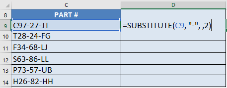
So place in the number 2 (as it is the 2nd instance the dash is located):

=SUBSTITUTE(C9, “-“, , 2)

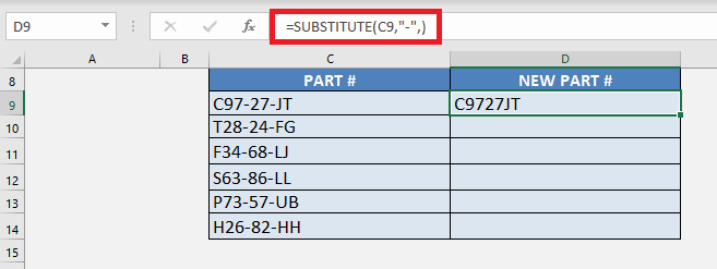
One thing you need to keep in mind is that if you ignore this argument, every occurrence of the old text will be changed to the next text.

Let’s try it!

=SUBSTITUTE(C9, “-“, ,)

 

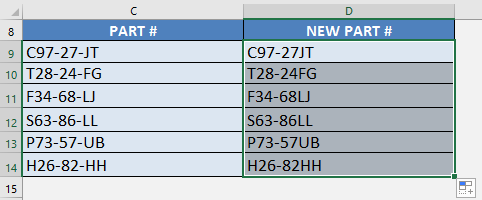
STEP 6: Do the same for the rest of the cells by dragging the SUBSTITUTE formula all the way down using the left mouse button.

Note that all of the parts are now changed to your new part values:

In this way, you can easily remove the 2nd occurrence of hyphens in Excel. This completes our tutorial on how to remove hyphen in Excel using the SUBSTITUTE function.

Following the steps mentioned above, you can easily change the nth occurrence of an old text with a new one.

 

Make sure to download our FREE PDF on the 333 Excel keyboard Shortcuts here: