Power Query or Get & Transform (In Excel 2016) lets you perform a series of steps to transform your Excel data. One of the steps it allows you to take is to rename a column using multiple methods.
I will show you how to do it step by step below!
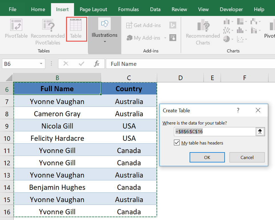
STEP 1: Select your data and turn it into an Excel Table by pressing the shortcut Ctrl + T or by going to Insert > Table
STEP 2: Go to Data > Get & Transform > From Table (Excel 2016) or Power Query > Excel Data > From Table (Excel 2013 & 2010)
Excel 2016:
Excel 2013 & 2010:
STEP 3: This will open up the Power Query Editor. Let us try the first method.
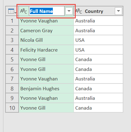
Make sure the Full Name column is selected. Either double click the column name or press F2.
Type in the new name Complete Name.
STEP 4: Let us now try the second method.
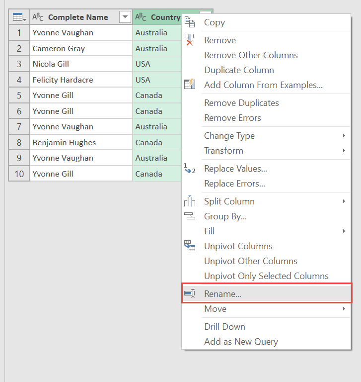
Right click on the Country column and select Rename.
Type in the new name Country of Residence.
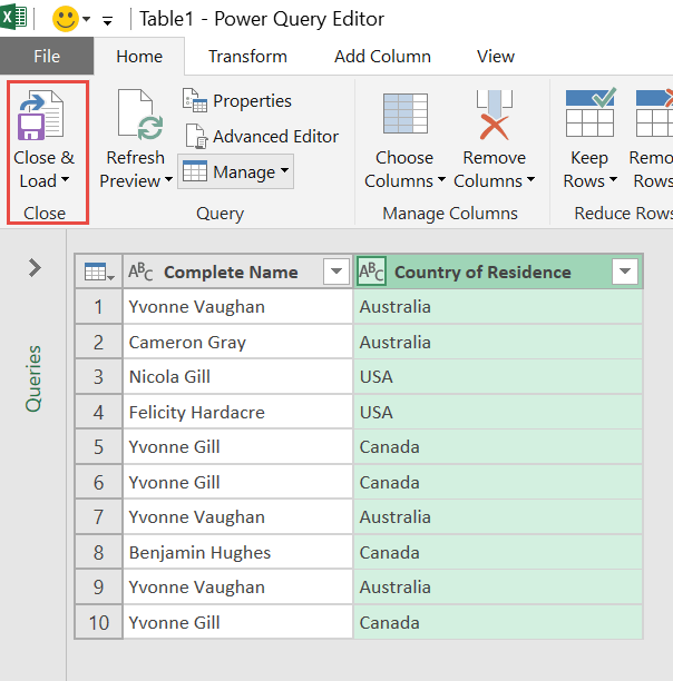
STEP 5: Click Close & Load from the Home tab and this will open up a brand new worksheet in your Excel workbook with the updated records!
You now have your renamed columns!
How to Rename a Column in Excel Using Power Query

Bryan
Bryan Hong is an IT Software Developer for more than 10 years and has the following certifications: Microsoft Certified Professional Developer (MCPD): Web Developer, Microsoft Certified Technology Specialist (MCTS): Windows Applications, Microsoft Certified Systems Engineer (MCSE) and Microsoft Certified Systems Administrator (MCSA).
He is also an Amazon #1 bestselling author of 4 Microsoft Excel books and a teacher of Microsoft Excel & Office at the MyExecelOnline Academy Online Course.

